I am using ControlSystems.jl with MonteCarloMeasurements.jl to analyse the step response of models with uncertain parameters and time delays. However, plotting the step response of a model with uncertain parameters vs. a model with uncertain time delays gives two different illustrations.
For example, running the following code,
sys = tf(1, [1, 1, 1]) * delay(Particles([0.1, 0.3]))
plot(step(sys, 0:0.01:5.0), lab=["delay=0.1" "delay=0.3"], ploty=false, plotx=true)
displays the below figure:
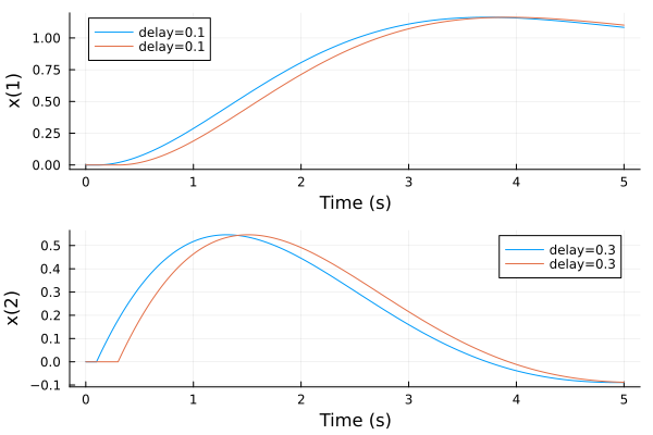
The above figure compares the step responses of the simple systems with time delays of 0.1s and 0.3s. I would like to produce the same plot but with two different model parameters (instead of time delays). However, the following code,
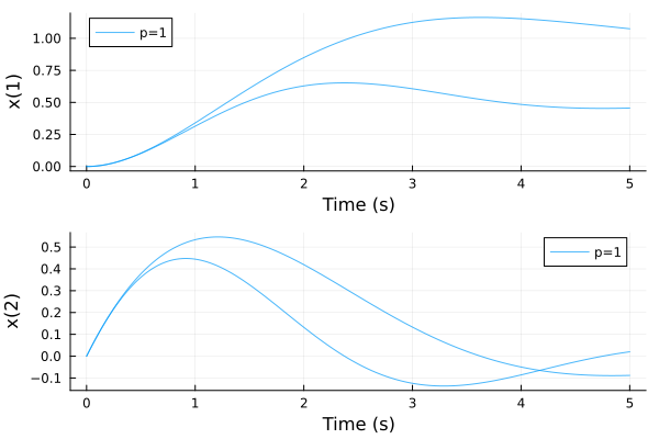
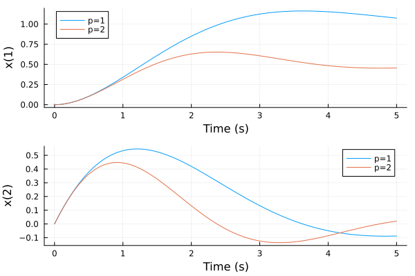
sys = tf(1, [1, 1, Particles([1, 2])])
plot(step(sys, 0:0.01:5.0), ploty=false, plotx=true)
displays the below figure:
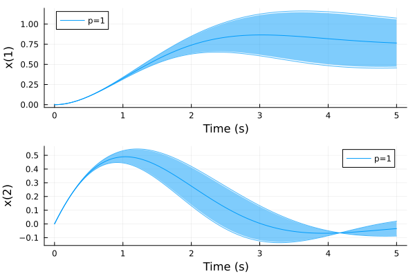
Here the result looks like a ribbonplot from MonteCarloMeasurements.jl, where for the time delay uncertainty the figure looks like a mcplot.
My question is why are these two results different? Is there a way to change how each one is displayed? For my use case, I prefer the first plot (where each parameter is plotted as a separate line). Any insight anyone has is greatly appreciated!