I’m pleased to announce my new package Desmos.jl! I’m a big fan of both Julia and Desmos, and I created this package to bridge the gap between them.
Desmos is a fantastic mathematical tool for drawing graphs in a web browser, and Julia is specialized for scientific computing. Desmos.jl allows you to generate Desmos graphs directly from Julia, making it easy to visualize your computations interactively.
Demo
Try copying and pasting the following code in your favorite IDE!
using Desmos

state = @desmos begin
    @text "First example"
    @expression cos(x) color=RGB(0, 0.5, 1) color="#f0f"
    @expression (cosh(t), sinh(t)) parametric_domain=-2..3
end
In VS Code, it displays like this!

In Pluto.jl, it displays like this!

In Jupyter, it displays like this!

Wait, isn’t it easier to just access Desmos | Graphing Calculator directly…?
I understand that feeling. But there are many application examples!
More Usage Examples
More Complex Expression Examples
While many functions in Julia and Desmos are similar, there are subtle differences that can be frustrating.
The @desmos macro absorbs these differences and handles them nicely.
using Desmos

@desmos begin
    sin(x)
    a1 = 2
    gradient(sin(a1*x), x)
    sum(n^2 for n in 1:5)
    sum([n^2 for n in 1:5])
end
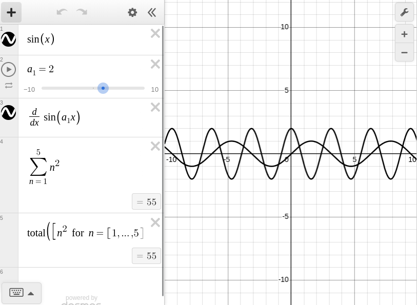
sin(x)becomes \sin(x)- The identifier
a1becomes a_1 using subscripts - Differentiation can be achieved using
gradient - The sum of a sequence becomes \sum
- The sum of an array becomes \operatorname{total}
See also the Function Compatibility section in the Desmos.jl documentation for details!
Using as a Plotting Library
Famous plotting libraries in Julia include Plots.jl and Makie.jl.
You can use Desmos.jl instead of these!
using Desmos
# x range from -10 to +10
xs = -10:0.1:10
# Create y arbitrarily
ys = xs.^2/10 .* randn(length(xs))
# Pack into a NamedTuple to render as a Desmos table!
nt = (; xs, ys)
@desmos begin
    @table $nt color="#ffaa00"
end

One advantage of using Desmos.jl is that you can interact with the plot results.
Polynomial Regression Example (Comparison of GLM.jl and Desmos.jl)
Let’s consider fitting a parabola to an arbitrary sequence of points in 2D.
using Random
rng = Xoshiro(42)

# Create a point sequence from sin
f(x) = sin(2x)

# x coordinates are random in the range (0,2)
x1 = 2rand(rng, 100)

# y coordinates are based on f(x) with random elements added
y1 = f.(x1) + randn(rng, 100)/10
In Desmos, you can easily perform regression using just the \sim symbol.
nt = (; x1, y1)
@desmos begin
    sin(2x)
    @table $nt color="#ff0000"
    @expression y1 ~ a*x1^2 + b*x1 + c color=RGB(0,1,1)
end
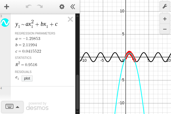
The coefficients are obtained as follows:
To do this in Julia, you can use the GLM.jl package, for example.
using GLM
nt = (; x1, y1)
fit(LinearModel, @formula(y1 ~ x1 + x1*x1), nt)
After execution, the following table is displayed, and you can confirm that the aforementioned coefficients are listed in the Coef. column.
y1 ~ 1 + x1 + x1 & x1

Coefficients:
────────────────────────────────────────────────────────────────────────────
                  Coef.  Std. Error       t  Pr(>|t|)   Lower 95%  Upper 95%
────────────────────────────────────────────────────────────────────────────
(Intercept)   0.0415522   0.0374524    1.11    0.2700  -0.0327805   0.115885
x1            2.11994     0.0865312   24.50    <1e-42   1.9482      2.29168
x1 & x1      -1.29853     0.0400957  -32.39    <1e-53  -1.37811    -1.21895
────────────────────────────────────────────────────────────────────────────
The advantages of using Desmos.jl would be:
- If you’re familiar with Desmos, you can edit formulas and check graphs in real-time
- You can experiment using Desmos’s intuitive GUI
- It can be used to verify results calculated with other Julia scripts
Of course, there are also disadvantages:
- You cannot bring Desmos calculation results back to Julia
- You cannot use objects defined in Julia (e.g., functions) directly in Desmos
It would be convenient to use GLM.jl for statistical analysis purposes and Desmos.jl for visualization/educational purposes as needed.
Newton Method Example
Let’s consider approximately solving the following nonlinear equations:
If you have an initial value sufficiently close to the solution, you can obtain an approximate solution through iterative Newton method calculations.
This nonlinear equation has four solutions, and if you prepare a background image color-coded by convergence destination, you can enjoy observing changes in convergence destination depending on initial value changes in Desmos.
using Desmos
# Image generated at https://github.com/hyrodium/Visualize2dimNewtonMethod
image_url = "https://raw.githubusercontent.com/hyrodium/Visualize2dimNewtonMethod/b3fcb1f935439d671e3ddb3eb3b19fd261f6b067/example1a.png"
state = @desmos begin
    f(x,y) = x^2+y^2-3.9-x/2
    g(x,y) = x^2-y^2-2
    @expression 0 = f(x,y) color = Gray(0.3)
    @expression 0 = g(x,y) color = Gray(0.6)
    f_x(x,y) = gradient(f(x,y), x)
    f_y(x,y) = gradient(f(x,y), y)
    g_x(x,y) = gradient(g(x,y), x)
    g_y(x,y) = gradient(g(x,y), y)
    d(x,y) = f_x(x,y)*g_y(x,y)-f_y(x,y)*g_x(x,y)
    A(x,y) = x-(g_y(x,y)*f(x,y)-f_y(x,y)*g(x,y))/d(x,y)
    B(x,y) = y-(-g_x(x,y)*f(x,y)+f_x(x,y)*g(x,y))/d(x,y)
    a₀ = 1
    b₀ = 1
    a(0) = a₀
    b(0) = b₀
    a(i) = A(a(i-1),b(i-1))
    b(i) = B(a(i-1),b(i-1))
    @expression L"I = [0,...,10]"
    (a₀,b₀)
    @expression (a(I),b(I)) lines = true
    @image image_url = $image_url width = 20 height = 20 name = "regions"
end
For simplicity, I omitted the background image generation this time, but it’s convenient to be able to work consistently in Julia from image generation to Desmos graph creation.[1]
Integration with Desmos Text I/O
Desmos Text I/O is a browser extension I created.

Graphs drawn in Desmos are internally handled as JavaScript objects.
By installing this extension, you can input and output these objects as JSON.
Desmos.jl provides a function called clipboard_desmos_state, which allows you to integrate with Desmos in the browser by copying and pasting via the clipboard.
using Desmos
# Enable clipboard button
Desmos.set_desmos_display_config(clipboard=true)
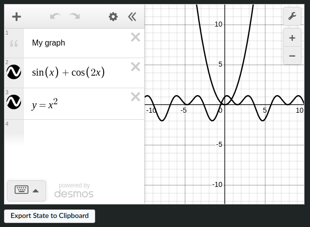
# Create a graph
state = @desmos begin
@text "My graph"
@expression sin(x) + cos(2x)
@expression y = x^2
end
# Copy graph to clipboard (also possible from the button below the graph)
clipboard_desmos_state(state)
Technical Details
Integration with JSON.jl
Desmos.jl handles Desmos graphs by representing them as JSON, which is the format used by the Desmos API.
The type output by the @desmos block is DesmosState, which directly corresponds to the JSON structure expected by Desmos. This clean mapping between Julia types and JSON was made possible by the excellent JSON.jl v1 package, released in October 2025. The new API provides great flexibility for defining custom serialization behavior, allowing Desmos.jl’s internal types to seamlessly match Desmos’s JSON format.
I’m grateful to the JSON.jl contributors for their work on this major release, which greatly simplified the implementation of Desmos.jl!
julia> using Desmos

julia> state = @desmos begin
           @text "First example"
           @expression cos(x) color=RGB(0, 0.5, 1) color="#f0f"
           @expression (cosh(t), sinh(t)) parametric_domain=-2..3
       end;

julia> typeof(state)
DesmosState
Desmos API
Given that the DesmosState type corresponds to JSON, how should we render it outside a browser?
This is made possible by the Desmos API! The library is published as a js file, and anyone can easily embed and use Desmos graphs on their own web pages.
At the time of writing, the API version in the latest documentation is v1.12, the API version used at Desmos | Graphing Calculator is v1.11, and the version with a publicly available API key in the documentation is v1.10.[2]
Desmos API appears to be free for personal use and paid for commercial use. I’m developing Desmos.jl as a hobby, so it’s free - thank you![3]
Implementation of Base.show
Now that we know Desmos graphs can be embedded in HTML files, how can we embed them in VS Code, Pluto.jl, or Jupyter output?
Answer: Just define the following two methods:
Base.show(io::IO, ::MIME"text/html", state::DesmosState)Base.show(io::IO, ::MIME"juliavscode/html", state::DesmosState)
By defining these, plots will be displayed as mentioned above.
Long live multiple dispatch!!!
Custom latexify Implementation
Now, in the JSON representing Desmos graphs, each formula block is saved in LaTeX format. Desmos’s rendering engine internally parses this LaTeX nicely to draw graphs.
In Desmos.jl, to implement the @desmos macro, I needed to convert from the Expr type to the LaTeXString type.
One Julia package that meets this requirement is Latexify.jl, and I used this package before, but now it’s a custom implementation.
julia> using Latexify, Desmos

julia> ex = :(sin(x))
:(sin(x))

julia> Latexify.latexify(ex)  # Latexify.jl includes $ and spaces
L"$\sin\left( x \right)$"

julia> desmos_latexify(ex)  # Aligned with Desmos's standard format
"\\sin\\left(x\\right)"

julia> ex = :([1,2,5])
:([1, 2, 5])

julia> Latexify.latexify(ex)  # Latexify.jl converts to column vector notation
L"$\left[
\begin{array}{c}
1 \\
2 \\
5 \\
\end{array}
\right]$"

julia> desmos_latexify(ex)  # In Desmos, [] is treated like an array
"\\left[1,2,5\\right]"
Macro Implementation
Things that start with @ like @desmos are Julia macros.
This macro implementation required some ingenuity:
- When
$is used inside@desmos, the contents of variables are expanded @expression,@table, etc. can be used inside@desmos, but they are not exported from Desmos.jl- In
@expression, etc.,colorand other parameters can be set like keyword arguments
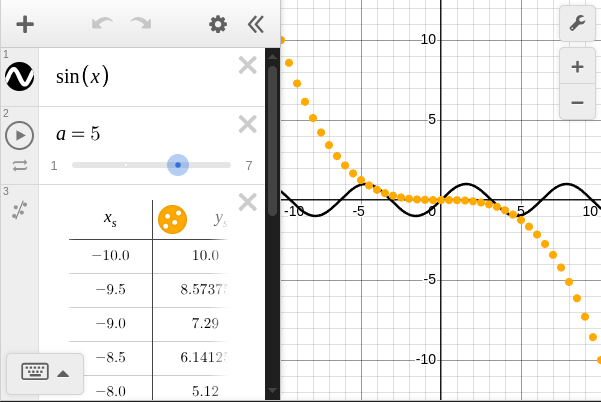
using Desmos
xs = -10:0.5:10
ys = -xs.^3/100
nt = (; xs, ys)
@desmos begin
    sin(x)
    @expression a=4 slider=1:2:7
    @table $nt color="#ffaa00"
end
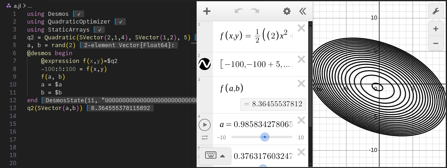
Rendering User-Defined Types in Desmos
In my package QuadraticOptimizer.jl, I define D-variable quadratic functions as Quadratic{D}, and it’s possible to use this with Desmos.jl.
using Desmos
using QuadraticOptimizer
using StaticArrays
q2 = Quadratic(SVector(2,1,4), SVector(1,2), 5)
a, b = rand(2)
@desmos begin
    @expression f(x,y)=$q2
    -100:5:100 = f(x,y)
    f(a, b)
    a = $a
    b = $b
end
q2(SVector(a,b))
To use this type Quadratic{D} in Desmos.jl, only the following two methods are defined:
desmos_latexify(::Quadratic{1})desmos_latexify(::Quadratic{2})
Adding these methods can be achieved as a package extension, so feel free to use it for user-defined types!
Things That Are Probably Fundamentally Impossible to Implement
The following items would be convenient if they could be realized in Desmos.jl, but I think they’re probably impossible:
- Treating functions defined in Julia as Desmos functions
- Obtaining Desmos calculation results on the Julia side
- Executing Julia functions via actions defined in Desmos
Future Plans
- Add support for more Desmos features
- Enable 3D plotting
- Enable handling of complex numbers
- etc.
- Use Desmos.jl as a backend for Plots.jl (if possible)
A script for generating background images is available at GitHub - hyrodium/Visualize2dimNewtonMethod. ↩︎
In the v1.10 documentation, the API key is listed in the first code example. In the v1.11 and later documentation, there is no API key listed, and application is required for use. ↩︎
Although Desmos.jl is published under the MIT license, commercial use is restricted regarding API usage. Please be aware. ↩︎
