[ANN] ConvolutionInterpolations.jl: Smooth multi-dimensional high order of accuracy interpolation

[stevengj]

@NikoBiele

Kernels which yield nearest neighbor, linear, cubic, quintic etc. interpolation, all the way up to highly smooth C11 continuous 7th order accurate 13th degree interpolation (I derived these highly accurate kernels myself using SymPy).

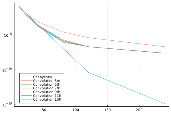
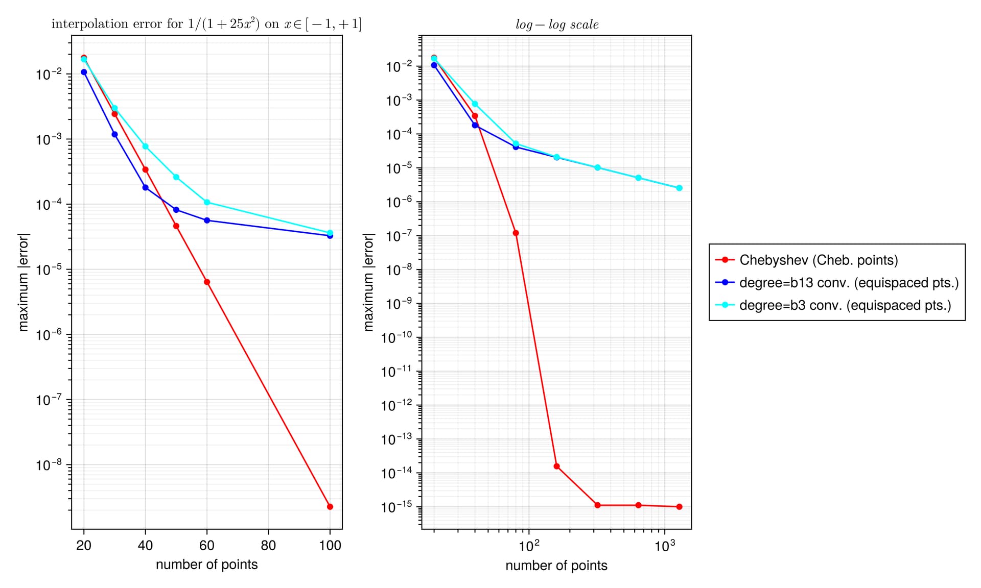
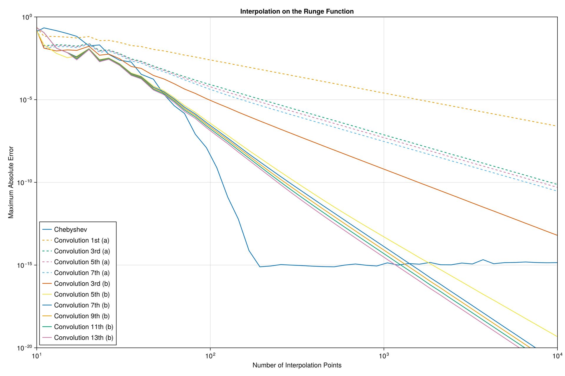
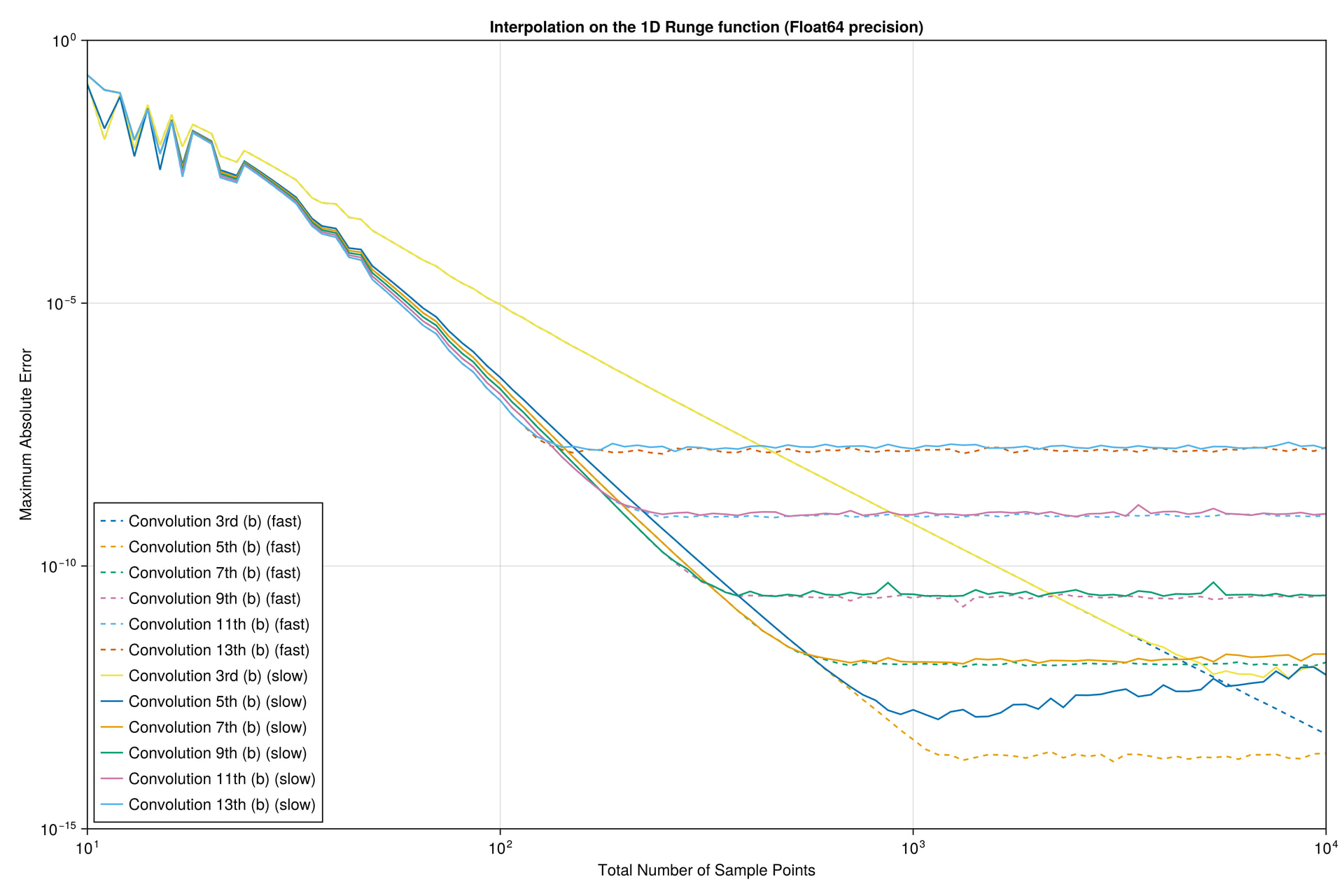
I did a quick test with these interpolants on the Runge test function 1/(1+25x^2) on x \in [-1,1], looking at the maximum error maximum(abs.(interp.(x) .- exact.(x))) at 10^5 equispaced points x = range(-1, 1, length=10^5), plotting the convergence as a function of the number of interpolation points.

I found something strange to me: if I compare your degree-13 kernel :b13 to the degree-3 kernel :b3, the former is more accurate at first, but asymptotically they have the same accuracy. Why doesn’t the high-order kernel converge faster?

Am I missing something?

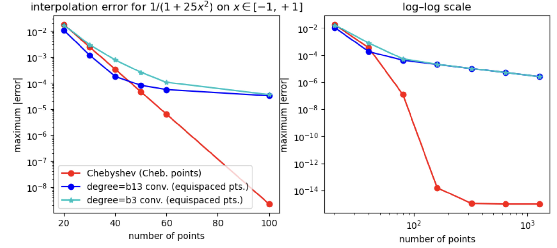
For comparison, I’ve also included the FastChebInterp.jl polynomial interpolation using the same number of Chebyshev points, which converges exponentially with the number of points. Of course, there are lots of circumstances where you are forced to use equispaced points and cannot use Chebyshev points!

Code

using ConvolutionInterpolations, FastChebInterp

runge(x) = inv(1+25x^2)
xf = range(-1, 1, length=100000)
yf = runge.(xf)

ns = [20,30,40,50,60,100]
errs = [
    begin
        xc = chebpoints(n, -1,1)
        c = chebinterp(runge.(xc), -1,1)
        xr = range(-1,1, length=n)
        itp3 = convolution_interpolation(xr, runge.(xr); degree=:b3);
        itp13 = convolution_interpolation(xr, runge.(xr); degree=:b13);
        maximum(@. abs(c(xf) - yf)), maximum(@. abs(itp3(xf) - yf)), maximum(@. abs(itp13(xf) - yf))
    end for n in ns
]

nslog = [20,40,80,160,320,640,1280]
errslog = [
    begin
        xc = chebpoints(n, -1,1)
        c = chebinterp(runge.(xc), -1,1)
        xr = range(-1,1, length=n)
        itp3 = convolution_interpolation(xr, runge.(xr); degree=:b3);
        itp13 = convolution_interpolation(xr, runge.(xr); degree=:b13);
        maximum(@. abs(c(xf) - yf)), maximum(@. abs(itp3(xf) - yf)), maximum(@. abs(itp13(xf) - yf))
    end for n in nslog
]

using PyPlot
figure(figsize=(10,4))

subplot(1,2,1)
semilogy(ns, getindex.(errs, 1), "ro-")
semilogy(ns, getindex.(errs, 3), "bo-")
semilogy(ns, getindex.(errs, 2), "c*-")
xlabel("number of points")
ylabel("maximum |error|")
legend(["Chebyshev (Cheb. points)", "degree=b13 conv. (equispaced pts.)", "degree=b3 conv. (equispaced pts.)"])
title(L"interpolation error for $1/(1+25x^2)$ on $x \in [-1,+1]$")

subplot(1,2,2)
loglog(nslog, getindex.(errslog, 1), "ro-")
loglog(nslog, getindex.(errslog, 3), "bo-")
loglog(nslog, getindex.(errslog, 2), "c*-")
xlabel("number of points")
#ylabel("maximum |error|")
#legend(["Chebyshev (Cheb. points)", "degree=b13 conv. (equispaced points)", "degree=b3 conv. (equispaced points)"])
title("log–log scale")

[GunnarFarneback]

@NikoBiele

I think there may be some confusion about the methodology here.

I believe the confusion is less about methodology and more about terminology.

[NikoBiele]

Thank you for your insightful comment @stevengj

The explanation is that the higher order kernels suffer more under the precomputed kernels, at least for densely sampled signals (truncating the kernel to a fixed number of points rather than recomputing expensive polynomials for each call).
If you set fast=false you will see that kernels larger than :b3 converge faster than :b3, at least for the first few hundred samples (the :b3 is published in the paper I cited, it is 4th order, while mine are 7th order, based on when the Taylor series vanished during derivation).
However, I am still a bit puzzled that those curves ‘bend’ and asymptotically approach a limiting accuracy. I suspect this occur due to the limited order of the boundary conditions used, which ultimately end up limiting the accuracy.
Using higher order boundary condition is unfortunately not feasible in general, since in most cases this will make the interpolation not behave well.
On the other hand I’m very satisfied that there’s actually valid competition with Chebyshev at least for sparsely sampled signals (clearly not on densely sampled!).

[NikoBiele]

Code:

using ConvolutionInterpolations
using Plots
using FastChebInterp

runge(x) = 1 ./(1+25*x^2)
xf = range(-1, 1, length=10_000)
yf = runge.(xf)

ns = [10,20,40,80,120,240]
cerrors = []
itpb3_errors = []
itpb5_errors = []
itpb7_errors = []
itpb9_errors = []
itpb11_errors = []
itpb13_errors = []
for n in ns
    xc = chebpoints(n, -1,1)
    c = chebinterp(runge.(xc), -1,1)
    xr = range(-1,1, length=n)
    itpb3 = convolution_interpolation(xr, runge.(xr); degree=:b3, fast=false, kernel_bc=[(:quadratic,:quadratic)]);
    itpb5 = convolution_interpolation(xr, runge.(xr); degree=:b5, fast=false, kernel_bc=[(:quadratic,:quadratic)]);
    itpb7 = convolution_interpolation(xr, runge.(xr); degree=:b7, fast=false, kernel_bc=[(:quadratic,:quadratic)]);
    itpb9 = convolution_interpolation(xr, runge.(xr); degree=:b9, fast=false, kernel_bc=[(:quadratic,:quadratic)]);
    itpb11 = convolution_interpolation(xr, runge.(xr); degree=:b11, fast=false, kernel_bc=[(:quadratic,:quadratic)]);
    itpb13 = convolution_interpolation(xr, runge.(xr); degree=:b13, fast=false, kernel_bc=[(:quadratic,:quadratic)]);
    push!(cerrors, maximum(abs.(c.(xf) - yf)))
    push!(itpb3_errors, maximum(abs.(itpb3.(xf) - yf)))
    push!(itpb5_errors, maximum(abs.(itpb5.(xf) - yf)))
    push!(itpb7_errors, maximum(abs.(itpb7.(xf) - yf)))
    push!(itpb9_errors, maximum(abs.(itpb9.(xf) - yf)))
    push!(itpb11_errors, maximum(abs.(itpb11.(xf) - yf)))
    push!(itpb13_errors, maximum(abs.(itpb13.(xf) - yf))) 
end
plot(ns, cerrors, yscale=:log10, label="Chebyshev", dpi=1000, legend=:bottomleft)
plot!(ns, itpb3_errors, label="Convolution 3rd", dpi=1000)
plot!(ns, itpb5_errors, label="Convolution 5th", dpi=1000)
plot!(ns, itpb7_errors, label="Convolution 7th", dpi=1000)
plot!(ns, itpb9_errors, label="Convolution 9th", dpi=1000)
plot!(ns, itpb11_errors, label="Convolution 11th", dpi=1000)
plot!(ns, itpb13_errors, label="Convolution 13th", dpi=1000)

Plot:

[rafael.guerra]

Meta-comment: With such beautiful Julia code in this thread, it would be a shame to see the results displayed using PyPlot by a distinguished steward. Here is a beginner’s version using Makie:

Makie code

using GLMakie

f = Figure(size = (1000, 600))

ax1 = Axis(f[1, 1], yscale=log10, title = L"interpolation error for $1/(1+25x^2)$ on $x \in [-1,+1]$",
    xlabel="number of points",  ylabel="maximum |error|"
)
scatterlines!(ns, getindex.(errs, 1), color=:red, label="Chebyshev (Cheb. points)")
scatterlines!(ns, getindex.(errs, 3), color=:blue, label="degree=b13 conv. (equispaced pts.)")
scatterlines!(ns, getindex.(errs, 2), color=:cyan, label= "degree=b3 conv. (equispaced pts.)")

ax2 = Axis(f[1, 2], xscale=log10, yscale=log10, title = L"log-log\ scale",
    xlabel="number of points",  ylabel="maximum |error|"
)
scatterlines!(nslog, getindex.(errslog, 1), color=:red)
scatterlines!(nslog, getindex.(errslog, 3), color=:blue)
scatterlines!(nslog, getindex.(errslog, 2), color=:cyan)

Legend(f[1, 3], ax1)
f

[stevengj]

From your plot, there is barely any point in going beyond 5th order in your package?

[NikoBiele]

I agree, the improvement with going higher than degree 5 (quintic kernel) is actually quite small, compared to the growth in the computational burden (more equations+higher degree polynomials). I am grateful that you made me more aware of this fact and I will update the package and documentation so that kernel degree=:b5 will be the default, and recommend using it in the documentation. However, there is an improvement with higher degrees, especially for sparse sampling, even though it is not large, so I still believe it is justified keeping the higher degree kernels, even though they might not be worth the cost in many cases (especially in high dimensions).