[ANN] ConvolutionInterpolations.jl: Smooth multi-dimensional high order of accuracy interpolation

[NikoBiele]

Hi Julia people

I made this registered package for interpolation: GitHub - NikoBiele/ConvolutionInterpolations.jl: A Julia package for smooth high-accuracy N-dimensional interpolation using separable convolution kernels

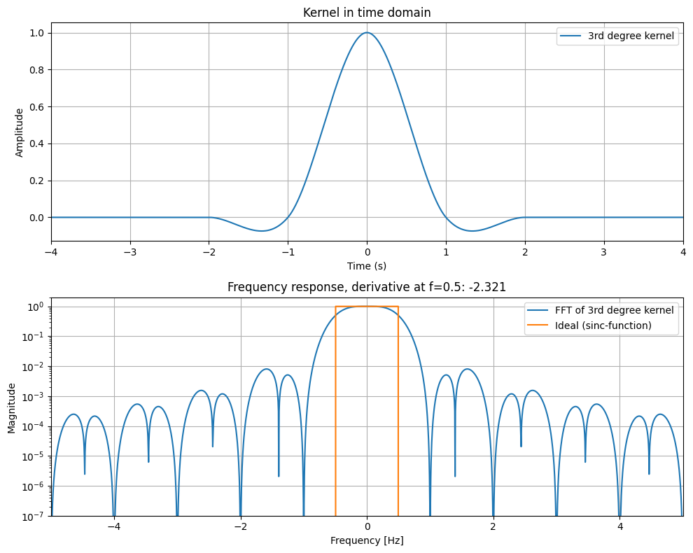
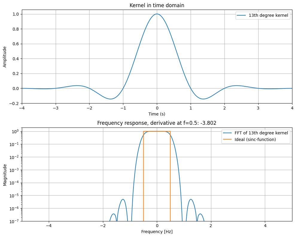
As visible from the plot below, it features a wide range of options in terms of accuracy: Kernels which yield nearest neighbor, linear, cubic, quintic etc. interpolation, all the way up to highly smooth C11 continuous 7th order accurate 13th degree interpolation (I derived these highly accurate kernels myself using SymPy).

Since convolution kernel-based interpolation depend on boundary conditions, I’ve made the package such that it auto-detects the most suitable boundary condition based on the data (linear, quadratic or periodic), but this behaviour can be customized, as explained in the readme.

The boundary handling is the main limitation of this package: When setting up the interpolator, each boundary is extrapolated to create the appropriate boundary condition, which is prohibitive in higher dimensions, due to the many boundary elements. Therefore, there is a trade-off between accuracy and high dimensionality: For high dimensions, using nearest neighbor og linear interpolation requires no boundary condition and should be efficient. As the degree of the polynomial kernel is increased, more boundary condition handling is necessary, increasing the time demand for setting up the interpolator. Also, for high-dimensional data, it is recommended to use the quadratic boundary condition since it is very efficient to evaluate compared to the default auto-detect behaviour.

This package has zero dependencies outside core Julia, so it should be stable over time and require minimal maintenance. I was very inspired by the API design of Interpolations.jl, since my package started out as a PR for that package.

I hope you will check out the package and find it useful.

[RoyiAvital]

What do you use for fast implementation of the convolution?

[NikoBiele]

Hi RoyiAvital,

Thank you for you response.

Convolution interpolation is based on a weighted average of the kernel functions, where the weights are the uniformly spaced data points in the neighborhood around the desired interpolated point. Since the kernel functions are independent of the data, for the fast implementation I simply precalculate the kernel functions at a specified number of points and store their values in a matrix. Then interpolation reduces to a single sorted lookup and a dot product between the data points and the relevant row in the matrix. Since sorted lookups are very efficient you can precalculate more points without a penalty.

[RoyiAvital]

I am not sure what you mean.
If data is equispaced then the interpolation is, as the name suggests, becomes a convolution operation.
Since you did not use any other package, I was wondering how fast your convolution implementation.
Have you compared your implementation of 1D convolution to other implementation in the eco system?

For instance:

1. ImageFiltering.jl.
2. DSP.jl.
3. Optimizing Direct 1D Convolution Code.

[NikoBiele]

Hi again RoyiAvital.

Here’s what I mean:
The way convolution interpolation works in general is to make a convolution between the data points and a number of predefined polynomials (the kernel). Therefore, it is indeed a convolution, but it is not a convolution between two signals, but rather a convolution between the data and the kernel which is designed to make the interpolated signal continuous. The way I speed up this convolution is to precompute these polynomials at a specified number of discrete points, and then use lookup and scaling. This method takes advantage of the fact that one of the ‘signals’ (the kernel) is known beforehand (and constant in a non-dimensional sense). This approach would not be possible for general convolution between two unknown signals. I have not compared my method to those that you mention. But I have compared it to ‘Interpolations.jl’ and mine is slightly slower (but higher continuity). You are welcome to make this comparison yourself.

[marianoarnaiz]

Hi @NikoBiele
This looks very exiting. It is nice to see more N dimension interpolations.
One question for me is how well it handles scattered/sparse data?

[NikoBiele]

Hi marianoarnaiz,

Thank you for your message.
For my package to be applicable, the grid spacing must be uniform for each dimension (but can be different between dimensions). So it cannot handle truly scattered data. But my experience from testing on sparsely sampled trigonometric functions (down to 3 samples per period) is that it works well for these (and often better than cubic splines). Other than your question I’ve also answered this question in an issue on GitHub: Support for non-uniform grid? · Issue #3 · NikoBiele/ConvolutionInterpolations.jl · GitHub.

[NikoBiele]

I just wanted to mention that I updated this package a bit (no breaking changes).
I updated the readme to quickly show example usage in 1D and 2D.

Most importantly I updated the package with a new extrapolation boundary condition:
This extrapolation boundary condition I’ve called ‘Natural()’.

The way it works is like this:
Normally my package extrapolates the domain once in each direction (with a number of coefficients depending on kernel degree), to create boundary condition coefficients for the kernel, for use when interpolating close the to boundary.

What this new extrapolation boundary condition does is to instead of extrapolating once, it extrapolates the domain twice, and uses the outer ‘layer’ coefficients as boundary condition, but interpolates past the original ‘inner’ boundary with full continuity preservation, that is, with this boundary condition, none of the continuity of the kernel is lost at the transition to extrapolation.

If trying to interpolate past the first layer of coefficients, the package apply a linear extrapolation. This extrapolation method is superior in my eyes, due to the preservation of high continuity. However, since it doubles the number of necessary boundary coefficients it needs to be used with care, and it is most suitable for the lower dimensions, depending also on how many coefficients the chosen kernel has. In general, high degree kernels always generate more boundary condition coefficients.

To choose the extrapolation method used for the ‘inner’ layer, when using the ‘Natural()’ extrapolation boundary condition, choose between the following kernel boundary conditions: ‘linear’, ‘quadratic’, ‘periodic’ or ‘detect’. Then this kernel boundary condition will be applied as the ‘inner’ boundary layer and will preserve continuity and transition naturally into the linear extrapolation (with high continuity) from the ‘outer’ boundary and out to infinity (within floating point). I hope someone will find this useful.

[stevengj]

@NikoBiele

For my package to be applicable, the grid spacing must be uniform for each dimension

Doing high-order polynomial interpolation on equally spaced points is susceptible to Runge phenomena, no?

(As opposed to high-order interpolation from Chebyshev points, ala FastChebInterp.jl)

[NikoBiele]

Good question!

No, I have not observed Runge’s Phenomena with this package.

The interpolation quality improves all the way up to 13th degree polynomials.

You are welcome to confirm this yourself.

[stevengj]

I don’t have my laptop with me for the next few days, but I would try it on the famous example function 1/(1+25x^2) on [-1,+1].

This isn’t really a question of your code—it’s inherent to polynomial interpolation (if that is what you are doing) from equally spaced points, regardless of algorithm. If you don’t see a Runge phenomenon with this function, then you are doing something that is not an interpolating polynomial. (Note that if you have N equally spaced points, it is safe to fit to a polynomial with degree much smaller than N.)

The other thing to look for is an interpolation that improves exponentially with degree for analytic functions, which is a characteristic of Chebyshev interpolation.

[NikoBiele]

Hi again Stevengj,

Yes, I thought about your questions during the day.

Our packages seem to be doing two quite different things:
Your package works on Chebyshev points.

My package works on equispaced points.

Both have their merits.

However, if you start from points sampled uniformly, getting to Chebyshev points would require some form of interpolation, before applying your approach, which could generate inaccuracy, regardless of the subsequent accuracy of Chebyshev interpolation. Am I right?

My package works directly with uniformly spaced points. Therefore, any ‘intermediate’ interpolation is unnecessary, hence a potential source of inaccuracy is eliminated.

I think maybe you are not familiar with convolution interpolation, since you mention polynomial fitting. Convolution interpolation is based on a convolution between the kernel and the signal. The kernel is a specially designed piecewise polynomial which satisfy conditions which make the resulting interpolation smooth up to a desired continuity:

1. The kernel has a value of 1 at the origin.
2. The kernel has a value of 0 at all other integers.
3. It is symmetric around the origin.
4. It has as high continuity as you designed it to have (higher continuity = wider support).
5. The kernel is zero outside the support region.

The reason that kernel based convolution does not result in oscillatory Runge’s phenomenon is that it is fundamentally not polynomial fitting. All of the high order polynomials are in the kernel, and they are fixed. The reason that increasing the order can not result in Runge’s phenomenon is that the rate of change of the kernel (so to say) with a change in the order is very small, and the kernel keeps all of it’s fundamental properties. Convolution interpolation is just a weighted sum of a number of polynomials, where the data points are the weights and the number of data points used depend on the support width of the chosen kernel.

Furthermore, the kernel’s I designed have a very nice frequency response (Fourier Transform) (superior to those in the literature, measured by closeness to the sinc function, which is the theoretically ideal kernel (but has infinite support, so it is unpractical)), which is the reason they perform so well.

I can recommend reading the papers I cite at the bottom of my readme if you’re interested in the subject.

EDIT: Ah, looking more closely on your package, you also have the ‘chebregression()’ function, which I think is actually what comes closest to what my package does (unknown function). I would be interested in comparing. In the readme you mention that the number of points should be much larger than the order. This is a difference from mine, as you can see in my readme, my 13th degree polynomial kernel works well with just 3 to 4 points per period on pure sine wave samples. However, the explanation might be the fact that my package uses a boundary condition (extrapolated extra points).

EDIT2: Looking even closer I can see you need to specify a function to interpolate, correct? This appear to be a fundamental difference from my package: My package does not work with functions, it simply ‘guesses’ the curve between points. Often one does not know the function.

[stevengj]

@NikoBiele

Looking even closer I can see you need to specify a function to interpolate, correct? This appear to be a fundamental difference from my package: My package does not work with functions, it simply ‘guesses’ the curve between points. Often one does not know the function.

No, my package does not require you to know the function. It simply takes values at the interpolation points and interpolates in between.

However, in many applications you can choose the points at which you evaluate the quantity to be interpolated, in which case you are well off choosing Chebyshev points — then you can use a polynomial degree equal to the number of points - 1, even for millions of points, and it is extremely well behaved if the unknown underlying function is smooth.

Of course, one important application is when you have a program that can compute the function at any point, but it is expensive. Then you can evaluate it at a few Chebyshev points, form the polynomial interpolant (the “surrogate”), and use that instead of your expensive program.

Whereas if you are interpolating, say, experimental data, you should be cautious about overfitting noise with high-order interpolation.

Regression, on the other hand (which my package also supports) is very different: it is a curve “fit” that is not guaranteed to go exactly through the data points, unlike interpolation.

[NikoBiele]

That is cool! Then your package appear to be superior in most cases.

[stevengj]

@NikoBiele

Convolution interpolation is just a weighted sum of a number of polynomials, where the data points are the weights and the number of data points used depend on the support width of the chosen kernel.

A weighted sum of polynomials is still a polynomial, and hence should be susceptible to a Runge phenomenon if the degree + 1 equals the number of data points (i.e. if you are forming the unique interpolating polynomial) for equally spaced points.

(Sorry, typing all this on my phone so it’s hard to dig more deeply into what you are doing.)

[apo383]

My interpretation is that polynomials are not fitted for interpolation. Rather, each kernel has polynomial coefficients already chosen, subject to a bunch of conditions that include very little high frequency ringing within the support region. Those kernels end up being pretty smooth (think Gaussians but different shape), and the interpolation is just convolving the kernel against the sampled signal. If you’re satisfied that they’re smooth, then the interpolation will be acceptable.

From looking at abstracts referenced in the GitHub repo, it looks like the idea is approximate a box filter with polynomials. The higher-order kernels are “smoother” at low frequencies and do exhibit some ringing at high frequencies, but at very low amplitude. I guess the low-frequency behavior matters is thought to matter more.

[NikoBiele]

Yes apo383, I agree with what you said.

Below are some figures I made to compare the original published kernel (:a3 in my package) versus my best kernel (:b13) (wide support, not all shown). As you can see there is very little high frequency information in the FFT of the 13th degree kernel (:b13 in my package).

[NikoBiele]

I just tried to use FastChepInterp.jl and I cannot understand how to use ‘chebinterp()’ without knowing the function? If I don’t know the function I can only specify a range and the y-values? How would the interpolator ‘know’ which x-values to use? When I try to use the package, it appears that you do need the function, or at least the ability to sample at Chebyshev points? If I just specify uniformly spaced y-values I get poor results compared to my own package… So I guess for uniformly spaced points, I still prefer my own package.

[zdenek_hurak]

Although I confess I am not fluent with kernel methods, checking one of the two papers referenced by the OP, it appears that if the kernels are assumed polynomials, then they consider piecewise defined polynomials (and symmetric on top of that), which makes them look hat-like.

This then enforces the locality of the method and perhaps explains why it does not suffer the same problem as the global polynomial interpolation on a uniform grid.

[apo383]

@NikoBiele I believe you can interpolate arbitrarily sampled points with chebregression(x, y, [lb, ub,], order), with x and y vectors of data. They still recommend keeping the polynomial order low.

@zdenek_hurak in addition to locality, they have several constraints on the coefficients, plus a parameter that’s set to reduce ringing. This probably makes the higher order coefficients quite small.