The chebinterp function assumes that the x values correspond to Chebyshev points for the same range, as returned by chebpoints. This assumes you have the freedom to choose the abscissae of the data points to correspond to Chebyshev points, which is the best case for high-order polynomial interpolation of smooth functions (you can use order N-1 with N points and get exponential convergence with N).
The basic question is where you are getting your data from, and in particular whether you have any control over how it is sampled.
If you have some other distribution of x values, e.g. N equispaced points, then in general you need to use much lower order (than N-1) polynomial fitting, lower order splines, or some other interpolation scheme entirely (e.g. radial basis functions), in order to avoid Runge phenomena.
From my understanding of radial basis functions, you need to solve a linear system for the coefficients, based on the data, before you can interpolate. Convolution interpolation does not need to solve a linear system before it can begin to interpolate, and as such it may be considered a ‘local’ method, which is automatically smooth and consistent with the data. All of the linear solves have been done ‘beforehand’, when designing the kernels. On the other hand, my package do need to extrapolate the domain to create a boundary condition, which can be prohibitive in higher dimensions, since there are so many boundaries to extrapolate.
What is wrong with the following test that produces NaN?
f(x,y,z) = 1 / (25 * (x^2 + y^2 + z^2))

u = 0.:0.05: 1.0
x = [[0.15, 0.0, 0.37], pi*[1/4, 1/5, 1/6]]  # interpolate at these 2 points
Fx = [f(x...) for x in x]

using ConvolutionInterpolations

itp_3d = convolution_interpolation((u, u, u), W; degree=:b13)
W2 = [itp_3d(x...) for x in x]     # produces NaN!
Errors2 = Fx - W2
Fyi, with GridInterpolations.jl no NaN is produced:
using GridInterpolations

U = RectangleGrid(u, u, u)  	# rectangular grid
W = [f(x,y,z) for x in u, y in u, z in u]

W1 = interpolate.(Ref(U), Ref(W), x)    # OK, no NaN
Errors1 = Fx - W1
At least in 1d, it seems like your convolution kernels can be viewed as an RBF chosen so that the system matrix is the identity matrix for equispaced points, and so that your basis functions have compact support.
In higher dimensions, it sounds like your basis functions are separable products of 1d functions, which is more different from an RBF.
Hi Rafael,
I think you have division by zero at one corner of your domain? It is this error which feeds into the coefficients and then into your interpolation. I would recommend modifying the function or the domain.
@NikoBiele, OK, thank you.
As Julia didn’t complain about that one Inf nor the other package, I had (unrealistically) hoped this package would consume it.
If you had used a more local kernel (more compact/smaller), there’s a chance you could have avoided hitting those NaN’s at the boundaries. For example if you’d used nearest neighbor (:a0) or linear (:a1) you likely would not have had that NaN returned, since those only use the points closest to the interpolation. But since you chose the widest possible kernel, the 13th degree polynomial (:b13), it is using a large amount of points to evaluate the interpolation. Therefore it included the NaN at the boundary and you got the NaN returned. From my perspective that is actually a good thing, since this would let you catch errors, rather than having them go unnoticed.
It is actually not a product, but a weighted sum, where the weights are the data points.
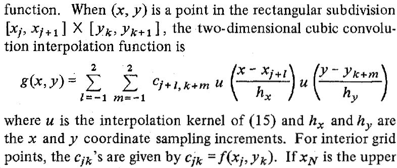
In 2d, for the cubic kernel, the sum is formulated as (same paper as the kernel above):
using ConvolutionInterpolations

f(x,y,z) = 1 / (25 * (x^2 + y^2 + z^2)+1e-12) # add some small constant
u = 0.:0.05: 1.0
W = [f(x,y,z) for x in u, y in u, z in u]
x = [[0.15, 0.0, 0.37], pi*[1/4, 1/5, 1/6]]  # interpolate at these 2 points
Fx = [f(x...) for x in x]
itp_3d = convolution_interpolation((u, u, u), W; degree=:b13)
W2 = [itp_3d(x...) for x in x]
Errors2 = Fx - W2
The floatmax(Float64) value you’re using is 1.79*10^308 which is an astronomically large number. The reason that you see a NaN is that the code is trying to extrapolate the domain past that singularity to create a boundary condition. All that the code see is that your domain is increasing towards the singularity, so it is trying to increase even further, hence end up producing NaNs. If you insist on including a singularity in your domain I recommend using linear interpolation.
@NikoBiele, thank you.
Replacing the single singularity by any number |x| ⪅ 1e10 seems to produce basically identical (good) results. A single data outlier is not a problem for the example given.
Remember that if you’re simply ‘replacing’ the singularity you’re not being entirely fair to the interpolation:
If you feed the interpolation a domain with a ‘replaced’ value, you’re essentially comparing two different functions, since the ‘replaced’ value will propagate into the domain through the interpolation.
Therefore I recommend to instead change the function (like I did above). Otherwise you’re comparing two different things.
The sum you wrote down is exactly what I said: the basis functions are products of 1d basis functions. That is, you have a tensor product of convolutions.
If I remember the literature correctly, this approach to interpolation defines a continuous kernel (of piecewise polynomials and compact support). This kernel is conceptually convolved with the discrete signal to produce a continuous result, which is then sampled in the interpolation points. In practice the computations are of course done to only compute the interpolated values and depending on the sampling pattern it may or may not be possible to reduce this to a discrete convolution with a constant kernel. In general it is not the case though and I see no indication that this package supports the special case, so comparisons to fast discrete convolution are not all that relevant.
That said, if speed is your main concern and you’re happy with 1D linear interpolation, then this package is probably not for you. We can benchmark it against a naive baseline:
using ConvolutionInterpolations
using BenchmarkTools
x = -10:1.0:10
y = x.^2
x_fine = -10:0.01:10
itp = convolution_interpolation(x, y, degree = :a1)
function interp1(x, y, xi)
    dx = x[2] - x[1]
    i = 1 + (xi - x[1]) / dx
    i1 = floor(Int, i)
    i2 = ceil(Int, i)
    alpha = i - i1
    return y[i1] * (1 - alpha) + y[i2] * alpha
end
Obviously this doesn’t say much about the performance of the more sophisticated interpolation schemes but I’m worried about the precision. Between 0 and 1 in this example, the closed form solution is the identity function and this looks much worse than can be expected.
Thanks a lot for your comment.
And thank you for testing my package.
This will allow me to explain a bit more in detail.
I understand your concerns about accuracy.
First of all, regarding your 1d example, this package was not designed primarily for 1d linear interpolation. I agree with you that other options are faster, for example Interpolations.jl, which support multidimensional linear interpolation. However, they do not support higher order interpolations in higher dimensions.
The reason you see those imprecise 1d interpolation results is due to the way that I designed this package.
You can avoid this issue entirely by setting the parameter fast=false (at the expense of speed), or you can reduce the precision loss by increasing the precompute parameter, for example setting precompute=10^6 will make the error go to the 7th significant digit. I made this design choice to allow the user to choose between using the full precision kernel (fast=false) or to increase the speed of the interpolation (by precomputing the kernel at discrete values), at a small expense of accuracy. When doing higher order interpolation of non-linear functions in N dimensions, this increase in speed is important, due to large number of points which need to be summed. But maybe I should explain this tradeoff more clearly in the documentation.
I’m under the impression that the assumption needed is a uniformly sampled grid which is what this package assume.
Just like BiCubic Interpolation can be done using convolution.
Am I missing something here?
You need to have both the data points and the interpolation points on uniformly sampled grids, and they need to have the same spacing, or integer multiples of the spacing. This package only assumes uniform grid for the data points.
I agree.
My false assumption was if the interpolation grid is a factor of the original data grid a convolution is used.
I guess the general solution is applied even for that case. So it remains a path for optimization.
Namely instead of setting arbitrary gird to calculate on just to define an interpolation factor.
@GunnarFarneback@RoyiAvital I think there may be some confusion about the methodology here. The package does implement convolution-based interpolation - specifically, for the case of 1d for example, you might ‘envision’ the convolution as overlaying the kernel (the hat) onto the data points, centered at the desired interpolation point (tip of the hat), and calculating the weighted sum of the kernel polynomials evaluated at the data points, weighted by the data points. Due to the constraints enforced during kernel design, this convolution operation automatically yields smooth interpolation. For more detail on the mathematical foundations, I’d recommend checking out the fundamental paper: R. G. Keys, “Cubic Convolution Interpolation for Digital Image Processing,” or the 1d implementation in ConvolutionInterpolations.jl: src/convolution_kernel_interpolation/convolution_kernel_interpolation_1d.jl (the ‘coefs’ are the data points). Happy to clarify any specific technical questions about the approach.