ODE solvers - why is Matlab ode45 uncannily stable?

EDIT: Turns out I was being stupid and the reason for the discrepancies in this case was indeed a trivial tolerance setting. However, I learned a lot in this thread, so thank you to all the contributors and especially to Chris, who I have kept from doing more important stuff.

Original Post starts here:

I am working with colleagues who work in Matlab. For parameter optimisation of ODEs I use Julia, because DifferentialEquation.jl is an order of magnitude faster, integrating the ODE set than Matlab, which makes the difference in getting an optimised parameter set in a few hours or in a few days.

So win there.

However:

  • in the Matlab models we use ode45 to solve the equations and the results are smooth
  • in Julia, using 4/5th order methods, I get oscillations, BS3() does work nicely.

My experience is similar in Python, where I need to drop the order of the algorithm to get an oscillation free result.

So my question is, why is Matlab’s ODE solver to uncannily stable for a 4/5 RK method? Julia and SciPy behave as I expect a higher order solver to behave in these cases, and I don’t mind using a 2nd or 3rd order method. But I need an argument to convince my colleagues that there is no problem in DifferentialEquations.jl

2 Likes

Actually: the 4/5 RK method is not that robust. I have an example in figure 7.6
of an older textbook that I wrote for an numerical-analysis UG course.

2 Likes

Do you have an example? Is it not just a default tolerance thing? MATLAB has a small dtmax which also can effect stepsizes.

2 Likes

I tought it may be dtmax, and I can get the Julia solver to give me a result that doesn’t have oscillations by reducing dtmax. But then Julia takes longer than Matlab (3x as long), while it normally would be 10x faster.

I was wondering if the speed-up should be that dramatic, since I assume ode45 is implemented in c, so should be fast as well.

Could it be that ode45 is quicker in lowering the time step to avoid oscillations?

Can you share an example?

1 Like

Your right-hand-side is implemented in Matlab, and it needs to be called multiple times per step, so that is generally the limiting factor in the speed for Matlab ODEs.

3 Likes

Obvious, if you say it like that :wink:

Did you double check that the right hand side gives exactly the same values on some random inputs? I haven’t seen an example that hasn’t come down to a translation error in this kind of thing yet (or someone modifying u, which MATLAB politely ignores due to copy on call). It would be highly helpful if you can get an example that runs with the comparison code, and verify with MATLABDiffEq.jl that MATLAB doesn’t have this issue (it auto-translates the ODE over to run in MATLAB, so that’s much easier to trust than the hand translation).

If there’s a case like that, my guess is that it might be that the PI-adaptivity gains of Hairer’s general schemes might be higher than Shampine’s, so I’d adjust some of the controller beta, but right now that would be speculation.

2 Likes

With modifying u do you mean something like:

...
u[2] = algebraic expression
...
du[2] = 0

I do that sometimes, but that is not the issue here. I have double checked the RHS, and at the moment it does indeed seem that the dt is the culprit. If I set dtmax manually, it does get more stable.

Here’s a jupyter notebook with some cleaned up minimal model that shows the behaviour. If I change dtmax (command commented out), so oscillation go away. Same if i choose BS() as the solver.

Unfortunately the automatic Matlab wrapper doesn’t seem to like the driving function, so I’ll have to implement exactly the same model in Matlab to have a 1:1 comparison.

EDIT:

I have created the Matlab model:

clear all
close all

time = [0:0.001:2];

figure(1)
plot(time, arrayfun(@i,time))

 
  Rc = 0.033;
  Rp = 0.6;
  C = 1.25;
  
  Ls = 0.01;
  
  Lp = 0.02;


options        = odeset('Reltol',1e-6);
P0 = [0 0];

tspan = [0 30];
tic
[t, P] = ode45(@(t,P) RHS_defn(t,P,Rc,Rp,C,Ls,Lp), tspan, P0, options);
toc

figure(2)
plot(t, P(:,1))
hold on
plot(t, P(:,2))


function i = i(t)
max_i          = 425;                   % current amplitude 
min_i         = 0.0;
T = 0.9;
systTime = 0.4 * T;
dicrTime = 0.02;

if rem(t, T) < (systTime + dicrTime) 
    i = (max_i-min_i) * sin(3.1419 / systTime * rem(t, T)) +min_i;
else
    i = min_i;
end


end


function dP = RHS_defn(t,P,Rc,Rp,C,Ls,Lp)

dP       = zeros(2,1);
dP(1) = -Rc / Lp * P(1) + (Rc / Lp - 1 / Rp / C) * P(2) + Rc * (1 + Ls / Lp) * didt(t) + i(t) / C;

dP(2) = -1 / Rp / C * P(2) + i(t) / C;

end

function didt = didt(t)
dt = 1e-3;
didt = (i(t+dt) - i(t-dt)) / (2 * dt);
end

I compare Tsit5 and BS3 with ode45 and found:

  • ode45 does give a result that features the notch and does not oscillate at the default settings

  • Tsit5 shows low frequency oscillations (longer than the period) and does not show the notch for the default settings

  • BS3 is “stable”, i.e. does not show the oscillations, but also does not show the notch with the default settings

  • Both Tsit5 and BS3 become stable and show the notch if I manually lower dtmax

Execution time: Matlab 90ms, Julia 15ms (but without the notch!), Julia lowdt 2s!

Julia Tsit5:

Julia BS3:

Matlab:

1 Like

DP5 is more dramatic. All of the solvers do give the “correct” result (or at least the same result), if I reduce dtmax (or use alg_hints=[:stiff]). Matlab seems to get dtmax right without intervention.

So the Julia solvers seem correct, but may be more aggressive in increasing the time-step.

I am aware that this is a particularly nasty driving function with two discontinuities (and the second one, the dicrotic notch, being a dramatic one). But this is one of the usual test cases for these models - and the dicrotic notch is a physiological effect (albeit less singular in real physiology).

This looks like a stiff problem. What happens if you use did solvers?

1 Like

Just edited the above post.

It is a stiff problem, and if I use alg_hints=[:stiff] then it does indeed work out of the box (with defaults).

Which brings me back to the original question: How on earth does ode45 (as a non-stiff solver) solve this without problems? What black magic are they using at Mathworks?

@time solutionTsit = solve(problem)
@time solutionTsitLowdt = solve(problem, Tsit5(), dtmax=2.5e-4)
@time solutionDP5 = solve(problem, DP5())
@time solutionDP5Lowdt = solve(problem, DP5(), dtmax=2.5e-4);
@time solutionDP5 = solve(problem,DP5())
@time solutionDP5Lowdt = solve(problem,DP5(), dtmax=2.5e-4);
@time solutionStiff = solve(problem, alg_hints=[:stiff]);
  0.006505 seconds (227.12 k allocations: 3.731 MiB)
  2.342365 seconds (76.22 M allocations: 1.288 GiB, 7.75% gc time)
  0.005744 seconds (210.63 k allocations: 3.370 MiB)
  2.394340 seconds (75.60 M allocations: 1.228 GiB, 16.53% gc time)
  0.005863 seconds (210.63 k allocations: 3.370 MiB)
  2.455301 seconds (75.60 M allocations: 1.228 GiB, 16.87% gc time)
  0.171663 seconds (5.58 M allocations: 89.534 MiB)

Matlab takes about 0.1seconds, so slower than the non-stiff Julia solvers, but faster than the stiff solver in Julia.

So I’m losing the argument to move to Julia at this point. Our real model is a lot more complex than this and has a similar problem.

Everybody is simply throwing ode45 at ODEs and gets away with it, without thinking twice whether it is actually the right algorithm. Why is it so uncannily robust?

EDIT: If I switch to ode15s in Matlab, then the execution time goes up to 0.3 seconds, which means Julia is faster again - not by as much as hoped, but good enough. However Matlab doesn’t seem to need the stiff solver here.

So just to clarify: The Julia (and Python, btw) solvers behave exactly as I would expect them to behave, the Matlab solver is performing in a way that it should not (at least as far as my understanding of higher order RK and stability goes).

Can you put the Julia code in the post? I can’t easily open up notebooks :sweat_smile:. I’ll take a look, or @YingboMa might find this one fun too.

Can you highlight what you mean by the oscillations though? I don’t see where you’re looking at in the picture (of Tsit5, DP5 is pretty clear and I think that’s just Hairer’s gain choice).

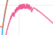
Edit: The feature that is critical is the notch, which all the small dt results and the stiff results show, but not the high dt results. This notch is a response to the driving function I, which looks like this:

ODEs:

function wk5(dP, P, params, t)

    #=

    The 5-Element WK with serial L
    set Ls = 0 for 4-Element WK parallel

    Formulation for DifferentialEquations.jl

    P:          solution vector (pressures p1 and p2)
    params: parameter array
                [ Rc, Rp, C, Lp, Ls ]


    I need to find a way to tranfer the function name as well
    for the time being we have to have the function in "I"

    =#

    # Split parameter array:
    Rc, Rp, C, Lp, Ls = params

    dP[1] = (
        -Rc / Lp * P[1]
        + (Rc / Lp - 1 / Rp / C) * P[2]
        + Rc * (1 + Ls / Lp) * didt(I, t)
        + I(t) / C
        )

    dP[2] = -1 / Rp / C * P[2] + I(t) / C

    return dP[1], dP[2]

end

Driving function (flow rate over time):

# Generic Input Waveform
  # max volume flow in ml/s
  max_i = 425

  # min volume flow in m^3/s
  min_i = 0.0

  T = 0.9

  # Syst. Time in s
  systTime = 2 / 5 * T

  # Dicrotic notch time
  dicrTime = 0.02


  function I_generic(t)
      # implicit conditional using boolean multiplicator
      # sine waveform
      (
          (max_i - min_i) * sin(pi / systTime * (t % T))
          * (t % T < (systTime + dicrTime) )
          + min_i
      )
  end

Central Difference (I used to use Calculus, but put this quick hack in to keep it consistent with the Matlab code:

function didt(I, t)
    dt = 1e-3;
    didt = (I(t+dt) - I(t-dt)) / (2 * dt);
    return didt
end

And finally, solving the thing:

# Initial condition and time span
  P0 = [0.0, 0.0]
  tspan = (0.0, 30.0)

  # Set parameters for Windkessel Model
  Rc = 0.033
  Rp = 0.6
  C = 1.25
  # L for serial model!
  Ls = 0.01
  # L for parallel
  Lp = 0.02

  p5 = [Rc, Rp, C, Lp, Ls]

I = I_generic

problem = ODEProblem(wk5, P0, tspan, p5)

dtmax = 1e-4

@time solutionTsit = solve(problem)
@time solutionTsitLowdt = solve(problem, Tsit5(), dtmax=dtmax)
@time solutionBS3 = solve(problem, BS3())
@time solutionBS3Lowdt = solve(problem, BS3(), dtmax=dtmax);
@time solutionDP5 = solve(problem,DP5())
@time solutionDP5Lowdt = solve(problem,DP5(), dtmax=dtmax);
@time solutionStiff = solve(problem, alg_hints=[:stiff]);

The oscillations in this case are low frequency, like this (Tsit5 default):

But I also get something like this on the other model. But this may actually be a different problem, since this doesn’t have the massive notch, and shows a high frequency oscillation.

Screenshot from 2021-06-18 16-05-15

This seems to be what I expect of a high order non-stiff solver, but, again, Matlab ode45 doesn’t show that.

Edit: Chris’ hunch that it is the time step seems to be correct, the Matlab solution has around 5985 steps for the 30 seconds (5278 for the stiff solver ode15s), while Julia has 193, 901, 173 for Tsit5, BS3, and DP5, respectively, and 4078 for :stiff.

It is to be expected that the time step chosen for dI/dt (function didt) is critical and that the notch can get missed (and it does). However, with only 200 time steps over > 20 cycles, it is not surprising that small scale features in the driving function are smoothed out (in particular since it’s dI/dt driving the inertia terms in the pressure response). The real driving functions will have a notch like that, but it will be smoothed out and differentiable, but still smaller than the chosen time step for the integration - so the problem shows on some of the measures curves as well (not as pronounced, and - worryingly - not as reproducible).

Am I correct in assuming that DP5 and ode45 are using the same algorithm?

So I have exported my org-mode file to Jupyter for naught? :wink:

BTW: Does Weave.jl support the plotly backend for Plots?

Here are a few lines of Julia code to convert notebook files to Julia: Export jupyter to .jl does not preserve markdown cells - #2 by stevengj

1 Like

I have looked into this a bit further and it seems to be a consistent bahaviour for my applications.

The main difference between most of the benchmarks I find on DifferentialEquations.jl and these problems is that I always have some term in the ODE that depends on a time-dependent parameter (in this case the flow rate I) and its derivative (in this case dI/dt).

I assume that the algorithms, as they are implemented in Julia are quite agressive in selecting a large timestep, which makes them very fast compared to Matlab.

This can be seen in the number of time steps used to solve a problem, which is about an order of magnitude smaller for Julia’s solvers compared to Matlab.

Since Julia uses time steps that are larger it will:

  • miss quick gradients in the driving functions (like the notch in this example, but also less extreme variations in them, like rapid acceleration or decay)
  • have a higher probability to phase shift, and thus have differing results from period to period (as seen in the results here)

So my assumptions are:

  • Where a set of ODEs in not driven by an exernal time-dependent function, but only by its own dynamic, the dynamic time step increase works, but the external driver cannot be predicted by the time step adaptation algorithm and thus my case fails with the default settings.
  • Matlab has to be more “robust” and has a less aggressive time step algorithm, so it does not exhibit these problems as much (it does, depending on the driving function, but in general you can get away with more).

I can get very good results with Julia, however:

  • I need to do time step convergence study and set dtmax manually
  • Julia loses the speed advantage, because that essentially means I am using a fixed time step (30000 steps in Julia, vs 5300 steps in Matlab in this case – 200000 steps in Julia, vs 23000 steps in Matlab for my real problem case). Julia is still a lot faster per time step, but since I need a lot more, it will become a lot slower than Matlab.

EDIT: For my real application ode45 (should be ode23s or ode15s, really, but ode45 does give the correct result - or at least the one I converge Julia to by reducing time step and tolerance) takes around 6 seconds for one integration. Julia, with manual dtmax reduction until converged, takes 45 seconds for that final run (plus the ones I need to find the maximum dt I can get away with).

EDIT: I believe Matlab is storing 4 data points for every time step (interpolated values between steps, so all the steps in Matlab would be 1/4.

1 Like

Cool you closer to Matlab behavior by lowering the tolerance?

Yes, if I lower tolerance to less than 1e-12 or 1e-16, then I get closer. But that means:

  • Julia needs much lower tolerances than Matlab (I use 1e-6 there as well)
  • Julia becomes slower than Matlab

In this case the problem may be a bit more complex due to the driving function — see my other post

EDIT: For my real application ode45 (should be ode23s or ode15s, really, but ode45 does give the correct result - or at least the one I converge Julia to by reducing time step and tolerance) takes around 6 seconds for one integration. Julia, with manual dtmax reduction until converged, takes 45 seconds for that final run (plus the ones I need to find the maximum dt I can get away with).

EDIT2: No, tolerance doesn’t seem to help. I did get a bit better in another case, but even lowering it to less than 1e-32 doesn’t solve this issue.

1 Like

I believe that ode45 employs some heuristics, in addition to the comparison between the different orders for accuracy, to direct the selection of the time step.