Since your ‘notch’ function is applied periodically & deterministically in time, you might want to implement it as a callback, which also serves to tell the solver “hey, I’m changing the state of the simulation, please time-step carefully around here”.
If you reach out to the Octave community, they may be able to shed some light on this. Presumably Octave’s ode45 must be very close to Matlab’s. Users of Octave will almost surely be aware of differences between Octave and Matlab when dealing with stiff problems. They may be able to guess the reasons for these differences. (short of looking at the Matlab source code, which I’m assuming is not open?)
Another quick trick that should work well for real-world driving functions: integrate dIdt within your differential equation:
P0 = [0.0, 0.0, 0.0]
 # ...
function wk5(dP, P, params, t)
    # the rest of wk5 is unchanged
	dP[3] = didt(I, t)
end
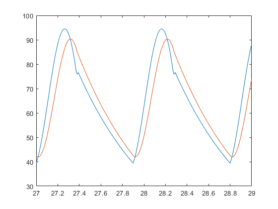
This accurately captures the notch behavior at all times with BS3() in ~1700 steps and takes ~30 ms on my machine.
Weird answers here… let’s pull this back to reality.
It wouldn’t be the tolerance. It would be the PI gains. PI controllers are used in the standard dopri methods, though from Shampine’s writings I would believe that the gains he uses are more conservative than the ones that Hairer uses. DifferentialEquations.jl DP5 matches Hairer’s Fortran dopri5 code to the dot: if you replace the ^ calculation with the C math library one you get essentially the same exact calculation (sans any compiler reordering of floating point calculations or muladd). There’s even a test on that:
where the tolerances are only higher than 1e-15 because of the aforementioned ^ calculation difference.
So it’s not surprising that DP5 and Python’s wrapper of the Fortran dopri5 have the same exact behavior since it’s by design. Tsit5 is created to have a slightly less aggressive controller because the algorithmic gains means it can be pulled back a little bit for stability.
Now when comparing against MATLAB remember that there are four “fake” points in there. Given the lack of interface options, Shampine knew he had to return arrays, but that would not plot well with the standard defaults. So four points from the 4th order interpolation are placed in the solve to fill out the array and look better for users, and that means when comparing the real behavior you need to subtract them.
So why is the PI adaptivity probably involved? These 5th order methods use advanced controllers in order to smooth the dt choices because that improves the stability on semi-stiff equations. Hairer’s are somewhat aggressive, which you can find here:
So what you really need to be doing is playing with different controllers. See the options on this:
https://diffeq.sciml.ai/stable/basics/common_solver_opts/#advanced_adaptive_stepsize_control
Given MATLAB is… MATLAB, I haven’t looked at the ode45 source (which I believe ships?) but if someone wants to take a peak and summarize here it would be interesting to know what controller parameters it uses.
[The other thing to mention is that MATLAB’s ode45 puts dtmax at 1/10th the interval limit, while DiffEq defaults to the interval limit, which is why that was my first guess. Lowering it so much was not what I intended you to do]
  ## Factor multiplying the stepsize guess
  facmin = 0.8;
  facmax = 1.5;
  fac = 0.38^(1/(order+1));  # formula taken from Hairer

    ## Compute next timestep, formula taken from Hairer
    err += eps;  # avoid divisions by zero
    dt *= min (facmax, max (facmin, fac * (1 / err)^(1 / (order + 1))));
Octave is only using I-control, so I would not think it would not be an algorithm that would match MATLAB stepwise, but if you want to do this one you’d do:
@time solutionDP5Lowdt = solve(problem,DP5(),qmax = 1.5, qmin = 0.8,
                               gamma = 0.38^(1/(order+1)),
                               controller = OrdinaryDiffEq.IController())
plot(solutionDP5Lowdt)
Wait a second…
In your MATLAB script you did:
options = odeset('Reltol',1e-6);
If you don’t change the default reltol then you get:
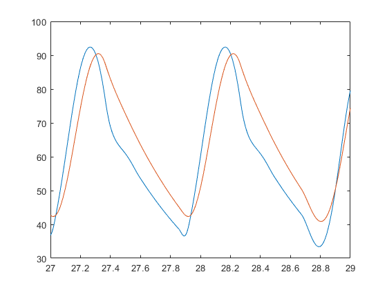
It’s only after you change to reltol=1e-6 that you get:
So it does require that you drop the reltol a little bit! And if you do that in Julia, it similarly works:
@time sol = solve(problem,DP5(),reltol=1e-6)
@time sola = solve(problem,Tsit5(),abstol=1e-12,reltol=1e-12)
length(sol) # 1368
plot(sol,tspan=(27.0,29.0))
plot!(sola,tspan=(27.0,29.0))
savefig("plot4.png")

which solves in 0.041426 seconds (1.50 M allocations: 23.584 MiB)
So why is your Julia code so slow? It’s because I_generic has a ton of non-constant globals in it, so it’s not type stable. So fix that and:
0.002944 seconds (8.27 k allocations: 870.594 KiB)
Ahh, that’s better.
Final code:
using OrdinaryDiffEq
function wk5(dP, P, params, t)

    #=

    The 5-Element WK with serial L
    set Ls = 0 for 4-Element WK parallel

    Formulation for DifferentialEquations.jl

    P:          solution vector (pressures p1 and p2)
    params: parameter array
                [ Rc, Rp, C, Lp, Ls ]


    I need to find a way to tranfer the function name as well
    for the time being we have to have the function in "I"

    =#

    # Split parameter array:
    Rc, Rp, C, Lp, Ls = params

    dP[1] = (
        -Rc / Lp * P[1]
        + (Rc / Lp - 1 / Rp / C) * P[2]
        + Rc * (1 + Ls / Lp) * didt(I, t)
        + I(t) / C
        )

    dP[2] = -1 / Rp / C * P[2] + I(t) / C
end

# Generic Input Waveform
# max volume flow in ml/s
const max_i = 425

# min volume flow in m^3/s
const min_i = 0.0
const T = 0.9

# Syst. Time in s
const systTime = 2 / 5 * T

# Dicrotic notch time
const dicrTime = 0.02


function I_generic(t)
  # implicit conditional using boolean multiplicator
  # sine waveform
  (
      (max_i - min_i) * sin(pi / systTime * (t % T))
      * (t % T < (systTime + dicrTime) )
      + min_i
  )
end

function didt(I, t)
    dt = 1e-3;
    didt = (I(t+dt) - I(t-dt)) / (2 * dt);
    return didt
end

# Initial condition and time span
P0 = [0.0, 0.0]
tspan = (0.0, 30.0)

# Set parameters for Windkessel Model
Rc = 0.033
Rp = 0.6
C = 1.25
# L for serial model!
Ls = 0.01
# L for parallel
Lp = 0.02
p5 = [Rc, Rp, C, Lp, Ls]

const I = I_generic
problem = ODEProblem(wk5, P0, tspan, p5)
@time solutionDP5 = solve(problem,DP5(), reltol=1e-6)
# 0.002944 seconds (8.27 k allocations: 870.594 KiB)
using Plots
plot(solutionDP5,tspan=(27.0,29.0))
savefig("plot1.png")
Nope, there’s an open issue on this in the Weave repo.
Ok, this is indeed embarrassing. I do drop the tolerance on Matlab by default, and was (don’t ask me why) under the impression that default in Julia would be 1e-6 anyway (should really have RTFMed).
So in this case it seems to be the solution. Unfortunately it isn’t in my real world case, but since the error there occurs in one of the values that is calculated from an algebraic equation, rather than one that is integrated as an ODE, it may be that I need to look at solving the ODE for that as well to avoid adding up the numerical errors on all ODEs.
I was playing with tolerances a lot on that code and it didn’t help, so I made an (unjustified) generalisation. I should know better, that’s the kind of thing I tell my students off for ![]()
Thanks a lot for that! This is extremely helpful. I have only been using Julia for a few weeks (I’m sure it shows in my code), and have thought about avoiding ambiguity in my variable types, but hadn’t thought about declaring constants as such - mostly laziness, I assume.
I’m used to working with 3D code, where there is no local adaptive time-stepping (there are some developments in the field, but it isn’t common place), so for a quick test, I simply dropped it down to see if all algorithms would converge to the same result (which they do, so that’s reassuring).
I will need to look into this. Apologies for not having read all the documentation. I thought it would be a quick fix - which it was, had I been more thorough.
So, apologies for wasting your time. But if it is a consolation, I feel that I learned a lot. I usually deal with 3D CFD, not 0D-models, so I am quite green in this field. And your explanations in this thread have helped me a lot to find where I need to look.
Thanks a lot for all your work on this. I have only really discovered Julia very recently, but I am hugely impressed by the whole DiffEq and SciML framework. We are looking to get rid of MATLAB (well I am and am trying to convince others - It helps that Julia is 1-indexed and that in many cases all you need to do is change function definitions and index parens) and move some of the Python code over - may be more difficult with Dutch collaborators ![]() - to avoid having to use C for the “real work”.
- to avoid having to use C for the “real work”.
Somewhat off-topic, but as a Dutchman working in HPC this remark makes me curious. Are we Dutchies more married to Python than other (EU) nationalities? ![]()
Since Python was invented by a Dutchman some of your compatriots see it as something of a national treasure ![]()
If I need to change these parameters, would typing the arguments in the function be similarly efficient?
ANSWER: Yes, more efficient, but not as efficient as const. Typed has about double the execution time over const - I assume the compiler simply hardcodes the constants in the machine code? So this realisation will be extremely useful for the optimisation setups, where I will definitely use const for everything that is not an optimisation parameter once we are out of the prototyping stage.
I used:
function I_generic(t::Float64, max_i::Float64, min_i::Float64, T::Float64, systTime::Float64, dicrTime::Float64)
....
end

I =  t -> I_generic(t, max_i, min_i, T, systTime, dicrTime)
to naively create a typed function.
Julia and MATLAB both use the same defaults of abstol=1e-6,reltol=1e-3.
Yes, for this you may want to look deep into the PID controller. @ranocha is the one who implemented the new controller system, and the reason was to make it easy to handle step limiters for CFL conditions.
Is a very nice paper on this, and the methods are documented as things like RDPK3Sp49. See:
https://diffeq.sciml.ai/stable/solvers/ode_solve/#Low-Storage-Methods
These kinds of methods will be able to impose more guarantees while achieving a higher dt on such a problem rather than something generic like DP5.
For more information on this, check out the 18.337 course notes on code optimization:
https://mitmath.github.io/18337/lecture2/optimizing

You can check the generated code and see that indeed const will specialize in there. Note that putting types in the signature won’t do anything here.
or this specific set of notes on optimizing code for differential equation solvers (with a PDE example):
https://tutorials.sciml.ai/html/introduction/03-optimizing_diffeq_code.html
Your actual issue is that the captured variables are still global until the function barrier. To stop that, I would use a callable type, like:
struct I_generic
  max_i::Float64
  min_i::Float64
  T::Float64
  systTime::Float64
  dicrTime::Float64
end

function (f::I_generic)(t)
  # access values via f.systTime
end

I = I_generic(max_i, min_i, T, systTime, dicrTime)
I(t)
As a starting point, do you know which settings would be the equivalent of MATLAB’s ode45 defaults? MATLAB is not perfect, and may lure us with a false sense of stability here, but I’d like to be able to reproduce the results.
DP5 with defaults should be rather close (as shown above) and it should react to tolerances similarly to ode45. PID controllers on SSP methods… there really is no clean comparison there, they are an entirely different algorithm with different behaviors ![]() .
.