Molly.jl - trying to understand di-atomic example

[BLI]

Thanks for lots of help on previous Molly.jl questions.

I’m trying to understand the " Simulating diatomic molecules example. I have re-structured the example to attempt to figure out the key ideas. See below (I skipped the cut-off of forces).

Questions:

1. Does my re-structuring make sense (see listing below)?
2. In spite of using Unitful.jl, it seems like “Data” must be specified in specific units. As an example, I get an error message if I provide sigma in pm instead of nm. Is this correct, i.e., specific units must be used?
3. Even though diatomic molecules are simulated, it seems like Lennard-Jones parameters (sigma, epsilon) for the atom is carried over and used for the molecule. Is this ok? Can I infer that if I, e.g., want to simulate \mathrm{N}_2, then I can use published LJ data for the molecule in the Atom specification?
4. Bonds between two atoms in a molecule seem to be specified via a potential energy for an ideal spring. Where can I find k_spring and r_spring for, say, \mathrm{N_2} and other molecules?
5. In the Molly.jl diatomic example, all atoms are initiated with a random velocity. Is this realistic when considering that half of the atoms are tightly bonded with the other atom in the molecule? Or this just done for simplification?

Import

#=
using Unitful
import Plots as plt
using Latexify
using LaTeXStrings
using Statistics
using Molly
=#

Data

# Atom data
# - Molar mass
M_atom = 10.0u"g/mol"
# - Lennard-Jones parameters
sigma = 0.3u"nm"
epsilon = 0.2u"kJ*mol^-1"
#
# Molecule data
# - Spring energy parameters between atoms 
k_spring = 300_000.0u"kJ*mol^-1*nm^-2"
r_spring = 0.1u"nm"
#
# Box for MD simulation
# - side of cubic box
r_box = 2.0u"nm"
#
# Thermostat
# - temperature 
T_ts = 100u"K"
# - atom/thermostat collision probability
Pr_ts = 2e-3
#
# Number of molecules
n_mols = 50

Setting up atoms & molecules

# Involved atoms 
atoms = [Atom(mass=M_atom, σ=sigma, ϵ=epsilon) for i in 1:2*n_mols]
#
# Bonds (spring potential energy) between atoms in molecules: k, r0 
bonds = InteractionList2Atoms(
    collect(1:n_mols),
    collect(n_mols+1:2*n_mols),
    [HarmonicBond(k=k_spring, r0=r_spring) for i in 1:n_mols]
)
#
# Interaction list
specific_inter_lists = (bonds,)

Setting particle box + placing molecules + molecule interactions

box = CubicBoundary(r_box)

# Coordinates for base atom in molecules
coords = place_atoms(n_mols, box; min_dist=sigma)
# Adding coordinates for skewed atom in molecules
for i in 1:n_mols
    push!(coords, coords[i] .+ [ustrip(r_spring),0.0,0.0]u"nm")
end

# Specifying velocity to atoms 
velocities = [random_velocity(M_atom, T_ts) for i in 1:2*n_mols]

# Pairwise interactions between molecules
pairwise_inters = (LennardJones(),)

Setting up system

# Subsampling of loggers
n_log = 10

sys = System(
    atoms=atoms,
    coords=coords,
    boundary=box,
    velocities=velocities,
    specific_inter_lists=specific_inter_lists,
    #pairwise_inters=pairwise_inters,
    #neighbor_finder=neighbor_finder,
    loggers=(
        temp=TemperatureLogger(n_log),
        pressure=PressureLogger(n_log),
        coords=CoordinatesLogger(n_log),
    ),
)

Simulating system

# Simulation times
# - Fixed timestep in DE solver
dt = 0.002u"ps"
# - Number of timesteps
n_dt = 1_000
# - Thermostat coupling time dt_ts; Pr_ts = dt/dt_ts 
dt_ts = dt/Pr_ts
#
# Specifying simulator
simulator = VelocityVerlet(
    dt=dt,
    coupling=AndersenThermostat(T_ts, dt_ts),
)
#
# Simulating System
# - Initial short simulation to compile simulation
simulate!(deepcopy(sys),simulator,20)
# - Full simulation
simulate!(sys,simulator,n_dt)

Plotting result

tvec = 0.0u"ps":dt*n_log:dt*n_dt

plt.plot(tvec,values(sys.loggers.temp); label="Molly logger")
plt.plot!(tvec,mean(values(sys.loggers.temp))*ones(size(tvec)); label="mean logger")
plt.plot!(tvec,temperature(sys)*ones(size(tvec)); label="Molly temperature")
plt.plot!(;xlabel="\\mathrm{time}", ylabel="T",unitformat=latexify,
            title="Diatomic Molly.jl example", frame=:box)

[jgreener64]

@BLI

Does my re-structuring make sense (see listing below)?

Removing the neighbour list, and hence the eligible matrix, is a problem because it means that atoms in the same molecule interact via the Lennard-Jones potential.

@BLI

Is this correct, i.e., specific units must be used?

You can use any units with the right dimension, but errors could arise if you use different units in different places.

@BLI

it seems like Lennard-Jones parameters (sigma, epsilon) for the atom is carried over and used for the molecule. Is this ok?

The Lennard-Jones potential is always applied to atoms, at least in Molly. The only thing defining the molecules is that there are harmonic bonds between the appropriate atoms.

@BLI

Where can I find k_spring and r_spring for, say, \mathrm{N_2} and other molecules?

Search online, or look in available force fields.

@BLI

In the Molly.jl diatomic example, all atoms are initiated with a random velocity. Is this realistic when considering that half of the atoms are tightly bonded with the other atom in the molecule? Or this just done for simplification?

Equilibration would sort out any negative effects from this. As I recall, though, the expected velocity distribution is independent of the potential definition.

[BLI]

Thanks for quick response. I have dug up some numbers for the bond model, but more generally for the Morse potential. I’ll check with the CRC handbook tomorrow – I think I have one edition in my office. As you suggest, I have also found numbers on the internet. And I found a pdf version of data for D_e (in Morse model) from the National Bureau of Standards (Darwent) + a web-version of a book by Herzberg.

---

OK - I’ll try to re-insert the neighbor list.

[BLI]

@jgreener64

Removing the neighbour list, and hence the eligible matrix, is a problem because it means that atoms in the same molecule interact via the Lennard-Jones potential.

To fully understand this…

# All pairs apart from bonded pairs are eligible for non-bonded interactions
eligible = trues(n_atoms, n_atoms)
for i in 1:(n_atoms ÷ 2)
    eligible[i, i + (n_atoms ÷ 2)] = false
    eligible[i + (n_atoms ÷ 2), i] = false
end

neighbor_finder = DistanceNeighborFinder(
    eligible=eligible,
    n_steps=10,
    dist_cutoff=1.5u"nm",
)

cutoff = DistanceCutoff(1.2u"nm")
pairwise_inters = (LennardJones(use_neighbors=true, cutoff=cutoff),)

The neighbor_finder just codifies which atoms are in the same molecule, right? While the pairwise_inters actually states that I should cut-off the Lennard-Jones interaction within the molecule?

So I need to remove the commenting on both of the lines:

    #pairwise_inters=pairwise_inters,
    #neighbor_finder=neighbor_finder,

---

I am also trying to understand how to set up the atom vectors… the way this is done in the tutorials is:

julia> [Atom(mass=1u"g/mol", σ=1u"nm", ϵ=1u"kJ/mol") for i in 1:2]
2-element Vector{Atom{Int64, Quantity{Int64, 𝐌 𝐍^-1, Unitful.FreeUnits{(g, mol^-1), 𝐌 𝐍^-1, nothing}}, Float64, Quantity{Int64, 𝐋, Unitful.FreeUnits{(nm,), 𝐋, nothing}}, Quantity{Int64, 𝐋^2 𝐌 𝐍^-1 𝐓^-2, Unitful.FreeUnits{(kJ, mol^-1), 𝐋^2 𝐌 𝐍^-1 𝐓^-2, nothing}}}}:
 Atom with index=1, atom_type=1, mass=1 g mol^-1, charge=0.0, σ=1 nm, ϵ=1 kJ mol^-1
 Atom with index=1, atom_type=1, mass=1 g mol^-1, charge=0.0, σ=1 nm, ϵ=1 kJ mol^-1

So both elements have index 1, and the index is not how you distinguish between the various atoms. So in defining the bonds,

bonds = InteractionList2Atoms(
    collect(1:(n_atoms ÷ 2)),           # First atom indices
    collect((1 + n_atoms ÷ 2):n_atoms), # Second atom indices
    [HarmonicBond(k=300_000.0u"kJ * mol^-1 * nm^-2", r0=0.1u"nm") for i in 1:(n_atoms ÷ 2)],
)

you use the location in the atoms vector to distinguish between then? Right?

---

What if I want to give the atoms different index?

julia> [Atom(mass=1u"g/mol", σ=1u"nm", ϵ=1u"kJ/mol",index=i) for i in 1:2]
2-element Vector{Atom{Int64, Quantity{Int64, 𝐌 𝐍^-1, Unitful.FreeUnits{(g, mol^-1), 𝐌 𝐍^-1, nothing}}, Float64, Quantity{Int64, 𝐋, Unitful.FreeUnits{(nm,), 𝐋, nothing}}, Quantity{Int64, 𝐋^2 𝐌 𝐍^-1 𝐓^-2, Unitful.FreeUnits{(kJ, mol^-1), 𝐋^2 𝐌 𝐍^-1 𝐓^-2, nothing}}}}:
 Atom with index=1, atom_type=1, mass=1 g mol^-1, charge=0.0, σ=1 nm, ϵ=1 kJ mol^-1
 Atom with index=2, atom_type=1, mass=1 g mol^-1, charge=0.0, σ=1 nm, ϵ=1 kJ mol^-1

I assume this would work just as well? Since setting up bonds does not use the index (but I may like to specify the index…).

[jgreener64]

@BLI

The neighbor_finder just codifies which atoms are in the same molecule, right?

It finds close pairs and applies exclusions to atoms that you don’t want to interact at all, in this case as they are bonded to each other.

@BLI

So both elements have index 1, and the index is not how you distinguish between the various atoms.

No, the index is not in general used but can be useful in some circumstances. The atoms are distinguished by their order in the vector. You can set the index to whatever you want. I can clarify this in the docs.

[BLI]

OK – I just had a “session” with the MS Copilot “shrink” on the meaning of DistanceNeighborFinder and DistanceCutoff vs. InteractionList2Atoms. So here is my understanding (I don’t fully trust this “shrink”…):

1. InteractionList2Atoms uses 2 vectors of atoms indices, and an intra-molecular bond potential. This is understood such that the bond potential applies to atom numbers in atoms with the same index in the 2 vectors. Copilot suggests that there is no cut-off of this bond potential.

2. The eligible matrix is for intra-molecular interaction… A simple example with 4 atoms and 2 molecules (green atoms are of the same element, red atoms are of the same but potentially different element):
   

   
   
   In my figure, ? indicates self-interaction. In the Molly diatomic example, the main diagonal is set to true (1), but I assume that the the inter-molecular potentials are not used for the main diagonal elements anyways, so I could probably just as well set the diagonal to false??

3. DistanceNeighborFinder uses the eligible matrix and refines this to only include molecules that are less than dist_cutoff apart? And specifies that this refined list of neighbors should only be updated every n_steps in the DE solver.

4. Furthermore, the DistanceCutoff further specifies a cut-off distance used by the actual inter-molecular potential (e.g., LennardJones). This cut-off distance should (normally) be slightly smaller than the one used in the DistanceNeighborFinder, partially to take into account that the list from DistanceNeighborFinder is only updated every n_steps.

My “shrink” session still leaves me with a couple of questions that MS Copilot is not very clear on…

• Will any of the cut-offs also apply to the intra-molecular bonds of the specific_inter_lists? MS Copilot states that the intra-molecular bonds are not cut-off, but that sounds weird as then there will less computational saving/less potential for parallelization on GPU:s, I would think. One possibility is that the intra-molecular bonds are not by default cut-off, but that if I specify a neighbor_finder value for the System constructor, the DistanceNeighborFinder cut-off is applied to the intra-molecular bonds for the false elements in the eligible matrix.

• If I simulate, say, di-atomic molecules, is it required to use a cut-off distance? MS Copilot says no, but that by not using cut-off distance, the results may be noisier.

[BLI]

OK – seems like for diatomic systems, the results are crazy unless I include cut-off. Don’t still know exactly how this works.

I chose the boundary box such that with ideal gas, I should get a “target” pressure of 100 bar at the given thermostat temperature.

I simulated di-atomic nitrogen. I chose cut-off in DinstanceNeighborFinder to 75% of the side of the boundary box, and the DistanceCutoff to 60% of the side of the boundary box - don’t know whether those are good coices. I extended the # samples to 10_000.

Temperature looks ok:

but the pressure looks strange (negative?):

If I reduce the specified target pressure to 10 bar, I get a positive average temperature, but it fluctuates quite a bit (from -10 to 20 bar).

Any ideas as to what would improve the results?

• shorter time step?
• a “better” initialization of velocities?
• using Morse potential instead of harmonic?
• etc.

---

Partially answering myself…

• using temperature 100K is perhaps somewhat close to the triple point of 63K?
• If I increase the temperature to, say, 300K, the pressure seems reasonable - even for a target of 100 bar.
• I tried to use the Morse potential instead of the harmonic potential. Difficult to say whether that helps.
• I tried to replace the random_velocity initiator with the maxwell_boltzmann initiator, but I get an error message – I assumed the same arguments as random_velocity, but that may be wrong.
• I tried with more molecules (going from 100 to 300). This predictably increased the simulation time (a factor of 9, more or less), but didn’t seem to change the results too much. I will need to check that further.

[jgreener64]

@BLI

Will any of the cut-offs also apply to the intra-molecular bonds of the specific_inter_lists?

No, specific interactions are not cutoff but tend to be short-ranged anyway. Looping over the specific interactions is fast, O(N) compared to O(N^2) for pairwise interactions without cutoff.

@BLI

If I simulate, say, di-atomic molecules, is it required to use a cut-off distance?

No, it is not required.

@BLI

Any ideas as to what would improve the results?

I don’t know much about the system, but try to match starting densities and temperatures from known experimental values.

[BLI]

Thanks!

I increase the thermostat temperature to 300 K, and targeted a pressure of 100 bar.

Shows variation in temperature for the last 10 ps of 20 ps simulation. Mean of logger (green line) is taken over the last 10 ps. Paler curves with 500 molecules and Morse bond, compared to 100 molecules.

Similar for pressure:

[BLI]

OK – now I am puzzled… I have used the mon-atomic and the di-atomic cases in the Molly.jl tutorial as basis, and simulated \mathrm{N_2}. And the result is strange.

In both cases, I use T_\mathrm{ts}=300\mathrm{K} as thermostat temperature, and I specify a “reference” pressure p_\text{ref} = 100\mathrm{bar}. Then I choose the number of molecules, and compute the necessary boundary box size from the ideal gas law to achieve thermostat temperature and reference pressure.

Case 1: I pretend that the \mathrm{N_2} molecule is rigid (a “pseudo-atom”), i.e., I do not model intra-molecular forces/potentials. I use the pseudo-atom Lennard-Jones parameters suggested in McQuarrie and Simon, \sigma_\mathrm{N_2} and \varepsilon_\mathrm{N_2}, for inter-molecular forces. No cut-off.

The result is as expected: an average temperature of ca. 298\mathrm{K} and an average pressure of ca. 100\mathrm{bar} (small variation from run to run due to random number generators).

Case 2: I assume a “flexible” molecule, with harmonic potential between the two \mathrm{N} atoms in the molecule. Next, for inter-molecular forces, I use \sigma_\mathrm{N} and \varepsilon_\mathrm{N} as found on the internet. These very closely satisfy \sigma_\mathrm{N} \approx \sigma_\mathrm{N_2}/2^{1/6} and \varepsilon_\mathrm{N} \approx \varepsilon_\mathrm{N_2}/4. I add neighbor_finder with appropriate cut-off distances, etc.

The result is really strange: an average temperature of ca. 302\mathrm{K} – fine – but the pressure is ca. 207\mathrm{bar}. Slightly more than twice of what it should be.

---

I have double and triple checked the code. But I don’t find any errors.

Next, I tried to re-do the simulation of Case 2, but this time with twice the size of the boundary box. In other words: as if I had half the number of molecules as I had in Case 1.

With this change of number of moles, the temperature is around 309\mathrm{K} (in the ballpark), while the pressure is (as expected) ca. 99\mathrm{bar}:

Here, the saturated colors indicate the result when I simulate Case 2 with with the same volume as for Case 1, while the pale colors indicate the result when I “cheat” and double the boundary box.

QUESTIONS:

• What is going wrong in my simulation?
• It is almost as if Molly.jl uses the number of atoms in the computation of the pressure, and not the number of molecules???
• Or is there something else going on?

[jgreener64]

If you are using the release version of Molly (0.22.3), try again with the new release that I will tag in the next few days. That adds more virial, and hence pressure, support.

If it still seems strange, post the code for the second case and I can take a look.

[BLI]

I’m using Molly v0.22.3. I will wait for the next release.

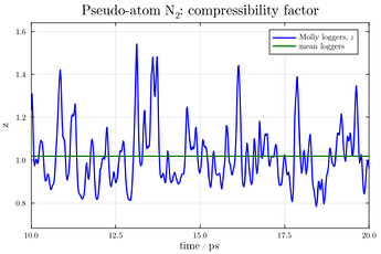
Btw. I computed the compressibility factor z for the “pseudo-atom” case (which gives correct pressure):

The ideal gas case is, of course, z=1, so the behavior should be close to ideal gas.

I guess the virial (\Xi, or \left<\Xi\right>) is proportional to z-1.

---

Two more indications of a problem with the number of molecules:

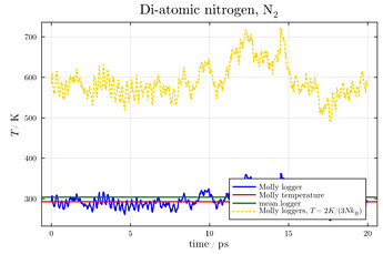
Temperature vs scaled kinetic energy in the di-atomic case:

The temperature (blue line) and the scaled kinetic energy (gold) should overlap exactly. They do in the pseudo-atomic case, but not here. If I, however, divide the kinetic energy by the number of atoms instead of molecules, then they overlap exactly.

Compressibility factor for the di-atomic case:

The correct value is ca. 1.0 (approximately ideal gas). The problem is that the pressure is twice as high as it should be – this indicates that the density is correct.