Basic Molly questions

I’m playing around with Molly.jl. Not really my field, but some colleagues worked with molecule simulations in the 1990s, so I have been exposed to the basic ideas. I also simulated a set of 5 Argon molecules in 2D, boxed in by a LJ-potential on the wall… (took some 10 minutes with MATLAB in 1994 or so, and some 5 s in Julia a few years back).


So I do the introductory example in the Molly.jl documentation. I have figured how to pick out the resulting vectors from the loggers + construct a time vector for the loggers:

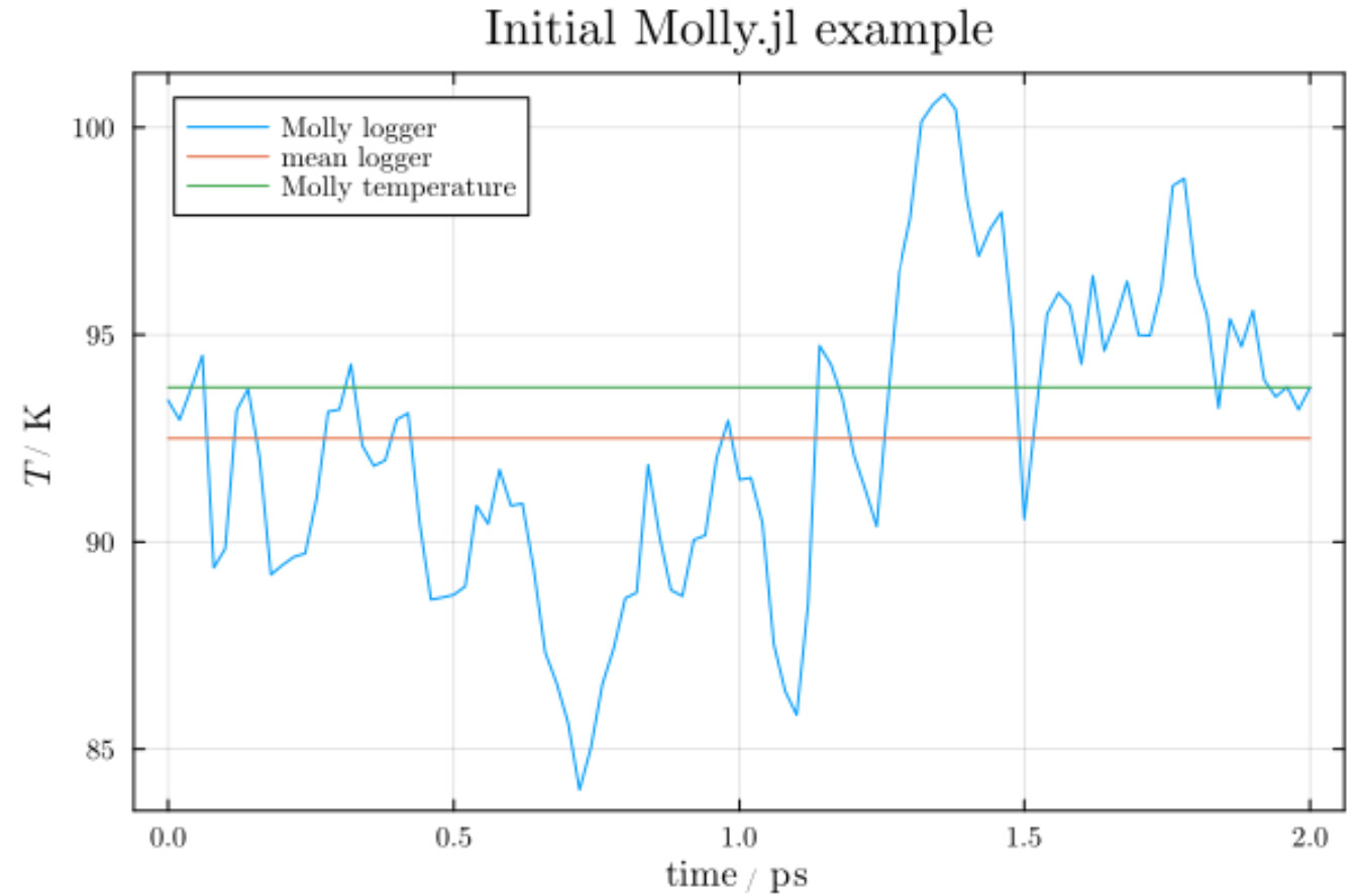
Question 1: I assume the variation in the temperature is a result of the Anderson thermostat not perfectly keeping the temperature at the specified temperature of 100 K?

Question 2: The red line is the mean of the logged temperature evolution. The green line is the result of using Molly’s function temperature(sys).

  • I’m curious as to why the green and red lines are different.

Question 3: The temperature is related to the “thermal energy” via the Boltzmann constant, right? Is the variation in temperature a result of variations in particle velocities? Or is it more complex? (Probably…)

I also logged the pressure:

Question 4: Same question as for temperature: is there a simple explanation for why the mean logged pressure and the pressure computed by pressure(sys) are different?

Question 5: The simulation with 100 molecules (atoms) and 1_000 time steps takes some 4 s on my laptop the first time I run the code, and virtually zero upon repeated simulation. Some simple questions:

  • how many molecules (and time steps) do I need to get reliable results if I want to compute the compressibility factor z from computed p, T, and molar volume?
  • in theory, T should be constant in these simulations, right? the variation is due to imperfect thermostat, right?
  • the molar volume is exactly given by the boundary volume and the number of molecules, right?
  • if I simulate more complex molecules, I still use keyword “atoms” in the System “instantiator”, right?
  • if I have mixtures of molecules, I just include two types of molecules in the “atoms” vector?

Stretching my understanding a bit… If I want to simulate two phase systems (vapor, liquid), do I need to add gravity to get the “liquid” to fall to the bottom? Is it possible to separate density for two (or more) phases?

1 Like

Yes, thermostats keep the mean temperature over time constant, not the instantaneous temperature which is calculated with temperature. The fewer particles you have, the more they will differ. Note how the green line matches the final blue point.

Yes, the Andersen thermostat can be thought of as randomly bumping particles to represent an interaction with the surrounding water bath. There will be variations with time, but the mean over time is conserved.

And the same answer, though you didn’t say whether you were using pressure coupling or not.

This is a hard question to answer generally; typically you would run repeats, discard an equilibration time from the start of each repeat, and look for convergence over the repeats.

See above about thermostats conserving the mean T over time.

Yes.

Yes, though you will probably need to pass in more interactions too.

The atoms vector doesn’t care about what molecule each atom is in. The molecules are defined by the interactions.

The issue is the boundaries. Molly supports periodic boundaries (atoms would fall through the floor) or infinite boundaries (atoms would float away). You might be able to have a wall exerting an interaction on the atoms, but that isn’t documented well. The Gravity interaction defines gravity between particles in the system. You would need a different interaction to add a constant gravitational force from earth, but it would only have a useful effect with a fixed wall.

Glad you are using Molly!

3 Likes

Yes, the Andersen thermostat can be thought of as randomly bumping particles to represent an interaction with the surrounding water bath.

Seems like temperature T is related to the average thermal energy per degree of freedom \langle E \rangle as

\langle E \rangle = \frac{1}{3}k_\mathrm{B}T

So without rotational coordinates, I assume the DOF is 3? This is the energy per particle, so to get the system energy, it is necessary to multiply with the number of particles?

If there are no particle interactions (ideal gas?), then I guess E is the kinetic energy of the particle? And if there is potential energy, some modification is involved?

  • Is this E the internal energy per particle?

In the ideal gas approximation (neglecting the LJ etc. potentials), I would guess that with temperature specified, one can compute what the size of the velocity should be – based on the above relation between E and T.

  • I’m guessing (speculating?) that this is how initial velocities are computed via random_velocity???

If the above is correct, then the Anderson (or other) thermostat is needed to adjust the velocities so that (i) the contributions of the potentials in E are taken into account, and (ii) possibly correcting for numerical errors in the differential equation solvers??

  • Are my guesses (i) and (ii) reasonable?

…how many molecules (and time steps) do I need to get reliable results if I want to compute the compressibility factor z from computed p, T, and molar volume?

I accept that that is difficult to answer in general. I seem to recall that my colleagues in the 1990s considered in the order of 1000 molecules. In principle, I guess one could have many molecules (say 1e3-1e4) and get a more accurate result, but also have fewer (say, 1e2-1e3) and do multiple simulations. With the latter strategy, perhaps it is also possible to infer a distribution of the computed quantities (say, pressure). Akin to Bootstrapping statistics.

Re: my question of the mean temperature/pressure over the logger values vs. the Molly temperature(sys) value

Aha – I see what you say: temperature(sys) and pressure(sys) seem to give the final value of the temperature and pressure, respectively.

To me, this makes sense if the computation of temperature and pressure gradually improves over the simulation time span.

  • But if there is no gradual improvement, wouldn’t then the mean make more sense?
1 Like

Just adding that liquid-vapor equilibrium has nothing to do with gravity, but with intermolecular forces. Liquid drops don’t boil for hanging at the roof.

1 Like

That is true :wink: . I was thinking more in terms of that from my experience, liquid gathers in the bottom of a volume, while the gas stays in the top of the volume. And I assume that has some relation to gravity. But I may be wrong.

These are very fundamental questions about statistical mechanics and simulations. If you want to see a Julia code with didactical purpose for a better understanding of that, take a look at:

Início · FundamentosDMC.jl Início · FundamentosDMC.jl

(The text is in Spanish, but browser automatic translation is generally very good)

The content there may answer many of your questions with associated simple implementations.

1 Like

Thanks! Will take a look. My Spanish is relatively rudimentary.

Of course, but that’s not what’s behind the phase equilibrium. In outer space the composition of the system would be the same (for the same pressure), but the liquid would be more like a floating drop attached to whatever wall is available, if any.

1 Like

As Leandro says, some of these questions can be answered by referring to statistical mechanics resources. Looking at the source code may also be helpful.

Velocities are drawn from the Maxwell-Boltzmann distribution, which only conserves averages.

The thermostat allows energy exchange with the “surroundings”, meaning that the mean temperature of the system matches that of the surroundings (the thermostat temperature).

Both the mean temperature and instantaneous temperature are useful, depending on what you want to do.

1 Like

OK – thinking it over a little bit more, I realize that the idea of liquid “falling to the bottom of the volume” is silly… since the boundaries are periodic, the “liquid clusters” would simply fall out of the volume and be replaced by similar clusters at the top.


So operating in one phase is conceptually much simpler. Still, doing phase equilibrium calculations (in particular for mixtures, say water - O2, where there are few experimental data available) would be interesting. There is a practical problem, though: from the experimental data I have seen (Pray et al., 1953), the mole fraction of O2 in the liquid is in the range of 1e-4-1e-3. So to get significant results, I’d guess there should be at least 10-100 O2 molecules in the liquid phase, requiring some 1e5 - 1e6 molecules in the simulations.

Phase equilibrium simulations are indeed hard. But depending on what you want, you can simulate a small system with two phases and normally in the time-scale of a simulation both phases will coexist. There is not time for actual equilibrium to take place. If you have a “small liquid phase” indeed the vapor phase will be just vacuum, but that is ok, for example, if you want to compute the transfer free energy of a small molecule (e. g. O2) from the liquid phase to the vapor phase - although for that you need specialized simulations to compute free energies.

2 Likes

For low-solubility gases (oxygen, methane, nitrogen) you’d probably want Widom test particle method or free energy perturbation to compute the standard Gibbs energy of hydration. From that, you get the ratio of concentrations of gas in vapor and liquid phases (Henry’s constant). And you’ll only need 1-10k particles for that.
Direct simulations with 1M molecules for such task are overkill and, more importantly, will take forever to equilibrate and get a good statistics. To ensure correct result, you’ll need to wait until (a) those 10 oxygen molecules get absorbed into water and (b) diffuse long enough so that you can get enough snapshots to reconstruct density distribution of oxygen in water, ensure it’s evenly distributed and compute the concentration.

3 Likes

Thanks. I wouldn’t know how to do that. I do have some correlation function for Henry’s constant for such gases (oxygen, nitrogen, hydrogen, etc.) from a paper publishes in 1960 – those correlations are based on experimental data. It would be interesting to test a molecule simulation result against those data, but my knowledge of statistical thermodynamics/molecular simulation is rudimentary. But I find the idea of using molecule simulations in tandem with classical thermodynamics models, Henry’s constant, etc. interesting.

If you’re interested, you may find some useful reviews and tutorials Living Journal of Computational Molecular Science.

3 Likes

Silly question, I guess: this Widom test particle method, does that work within Molly.jl? Or a different tool? I guess @lmiq uses his own code in his tutorial, and that is fine.

I have taught Model Predictive Control [MPC] in the past for many years, and I chose to never use MATLAB tools, etc., but instead let the students write the MPC code themselves – I think that gives more insight. If I where still teaching MPC today, I would, at least initially, let the students code the algorithm themselves (but: using a QP solver). Then, when they have understood the ideas, I would probably switch to a more polished tool such as Julia MPC packages. I would probably think similarly if I should ever teach something like thermodynamics and molecular simulations, but it all depends on the background of the students, I guess.

1 Like

@BLI For my very limiter understanding: does the QP solver in this context do energy minimization?

No. I was referring to QP solver used in MPC (model predictive control). I was just suggesting that I think it is good pedagogics to let student use simple implementations when they learn new theory (e.g., MPC), but that once the theory is mastered, it is more efficient to use a general tool. Likewise for molecule simulations, I would imagine: I think it is ok to let student program a simple molecule simulator (at least if they have some programming experience), but that when they understand concepts, it is usually more efficient to use a more general tool (which could, e.g., be Molly, or other tools).

1 Like

@BLI Clear. Agreed. Many thanks.

I’m not that familiar with this method, but from a quick look I think it could be done with Molly. An example would be a good addition to the documentation.

We are currently adding methods and documentation for MBAR, a different free energy method, to Molly.

If it were possible to compute, say, Henry’s constant for hydrogen and oxygen in water, that is relevant for fuel cells and water electrolysis. I have currently used correlations from the following paper from 1960:

[Don’t know whether it is a digitization error or a missing LHS negative sign in his Eq. 13; the negative sign is needed to replicate his Fig. 6]

The paper contains Henry’s constant correlations for O2, N2, H2, He, Xe, and CH4.

It would be interesting to compare these correlations with what one could get from, say Molly.jl.

I have also used Clapeyron.jl to compute fraction of H2 and O2 in liquid water. I really like Clapeyron; it is simple to use, and has loads of EoS:s. However, I suspect standard thermodynamic equilibrium calculations with the same EoS in both phases misses the solubility of H2 and O2 in liquid water by a factor of close to 50, at least compared to a few experimental data I have looked at, while Himmelblau’s H-correlation gives very accurate results for H2 and semi-good for O2 (non-perfect fit for O2 could be due to experimental data from 1952 or so at extremely high temperatures being less than ideal for my use).