Modeling wind power output random process across multiple geographical locations

[WalterMadelim]

Hello,

I want to model a vector stochastic process (may be decided according to historical observations).

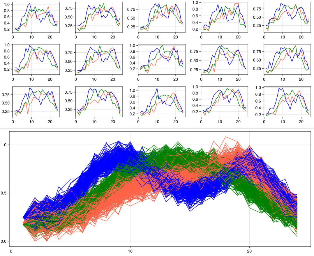
The length of the vector is N, which is the number of wind farms spreading in a power transmission network.
There are 24 hours in a day, denoted by T = 24.
I want to take account of temporal and spatial correlations.

A sample of the entire stochastic process should be a N-by-T matrix of wind power. Maybe the wind power of farm n at time t can be normalized to be in the interval [0, 1].

My minimum requirement about the uncertainty model is:

• I need the conditional distribution of column t+1 given the realization of column t (in the matrix above). (Yes, (I assume) it has Markov property)

My question is:

• Are there any advisable methods to build such an model realistically? (e.g. do I have to “transform” the numerics somehow (e.g. logistic function, z-score…)?)

---

Some additional notes:
My knowledge on statistics/regression/time series forecast is limited. And my knowledge on (engineering) wind power modeling is also zero.
I know there is a AR(1) model:

p_t = \mu + \Phi p_{t-1} + \epsilon_t

where \mu is a vector and \Phi is a matrix, both are weights to be decided on. And \epsilon_t is a stagewise independent error process (with multivariate normal distributions).

Since the \mu and \Phi do not depend on t, I naturally have a question here:

• Can I build 23 separate (vector) linear regression models? (the first one models the transition from t=1 to t=2, the second one models the transition from t=2 to t = 3…) Suppose I have enough historical data. So I can decide the weights separately for each transition with the respective data. Will this be feasible? What’s the difference compared with a naive AR(1) model?

And finally I want to ask:

• Are there any related mature julia packages in this regard?

[ufechner7]

It’s nice to see that more wind power researchers are using Julia!

Small remark: If you use LaTeX, enclose your formulas in $ signs.
This works nicely: \alpha \neq \beta

[technocrat]

Spoiler alert: NaCl needed

1. Normalization shouldn’t be required because you have a common dependent output variable, kWh.
2. Temporal autocorrelation is to be expected because wind doesn’t suddenly increase and decrease frequently.
3. Depending on how far about the wind farms are, spatial autocorrelation is also to be expected because they experience the same or similar wind velocities which may dominate differences in technologies among the farms. I haven’t found Ripley’s k in Julia, but rolling your own isn’t difficult.
4. y = f(x), so wind is y? Then you need time series linear regression, not ARIMA.
5. A good introductory text is Forecasting: Principles and Practice (3rd ed), although it’s R-based.
6. My impression is that the Julia time series ecosystem is no so well developed as R’s. You may want to consider doing your data prep in Julia and time series in R.
7. High-frequency time series modeling (hourly) generally produces better results using only the most recent data.
8. Seasonality in wind patterns needs to be accommodated and may indicate separate models. STL decomposition should be looked at, and a Fourier transformation of data, also.

[nilshg]

With Durbyn.jl we should get close to R’s forecast, so the Hyndman book might be doable in Julia now.

[WalterMadelim]

It appears that I’m not able to add Durbyn.jl automatically from within julia, currently.

It’s appears that julia’s ecosystem is not that strong for these applications. Might as well, indicating we have posterior benefits.

[technocrat]

It not in the registry. Have you tried

using Pkg
Pkg.add(url="https://github.com/taf-society/Durbyn.jl")

[WalterMadelim]

I haven’t tried.

I think there is a reason that the developers decided not to register.
I prefer to look into the theories at the current stage. And try if I can just write my own methods.

(I guess the realization is less an issue. Probably some optimization stuff. Julia is quite strong at optimization—we have JuMP.jl which I think has the greatest documentation.)

[technocrat]

Well, I, at least, don’t register if I’m not yet satisfied that a package is ready. As far as rolling your own, it’s great, so long as you verify against a known implementation. I like to use an R version as a reference to see if I get substantially the same results. Or if I don’t, there’s a reason why. For example, I have OLSPlots, which is slightly different from the plot method for R lm, which turns out to be due to differences with the implementation of loess in Julia.

[ufechner7]

@WalterMadelim

I think there is a reason that the developers decided not to register.

[ANN] Durbyn.jl — Time Series Forecasting in Julia

I plan to register the package in the first quarter of 2026. The low-level base models, such as arima(), auto_arima(), and ets() are now stable from an API perspective and will not undergo any breaking changes. I’ll continue to refactor and optimize their internals, but the external interfaces will remain consistent. At the moment, I’m introducing a formula interface grammar and building parallelization capabilities to support large-scale forecasting problems efficiently.

[Resul.Akay]

The main reason Durbyn.jl is not yet in the Julia General Registry is that we are still developing and iterating on a user-facing grammar. This takes time to experiment with and to converge on a design that feels intuitive for teaching and learning forecasting workflows.

Docs (dev): https://taf-society.github.io/Durbyn.jl/dev/

At the low-level model layer, the implementation closely follows the original R version, with some code-level enhancements. Because of these improvements, the Julia implementation may occasionally produce slightly different numerical results, but the core algorithms and model definitions are mathematically identical.

One example of such an enhancement is adding a safeguard against division by zero. In the reference implementation, we observed patterns like the following (illustrative example):

e[i] = (y[i] - f[0]) / f[0];

Here, no safeguard is applied when f[0] == 0. In Durbyn.jl, we handle this explicitly:

if abs(f[1]) < 1.0e-10
    f_0 = f[1] + 1.0e-10
else
    f_0 = f[1]
end
e[i] = (y[i] - f[1]) / f_0

This prevents failures when f[1] is zero (or extremely close to zero). However, it can also alter the likelihood surface along the optimizer’s path, which may lead to a different selected model in edge cases.

We did not find an explicit justification in the referenced papers for allowing a hard division-by-zero failure, so we opted for these kinds of robustness improvements.

[WalterMadelim]

About the e, y, f thing… Since I’m not that familiar with statistics, I have no idea where does this structure occurs. But is your if-else-end logic immune to the case when f[1] = -1e-10 + ϵ? in which case the denominator is an arbitrarily small positive number.

---

@Resul.Akay

user-facing grammar

I think I have some sort of this experience.
I’ve written code with JuMP for about two years, from my perspective I think the only functionalities that entail macros are building expressions and constraints, i.e. @expression, @build_constraint. But perhaps for consistency, they designed the whole set of @objective, @variable, @constraint. If I have some comments, that would be: I think macros for beginners are okay, but functional APIs are important equivalently (e.g. I don’t know how to create a JuMP variable without using @variable, which I find the design confusing).

---

I like this project. Hope to see a well-established package soon!
(I’d be more grateful if you have some experience to share on my wind power forecast model here😊)

[Resul.Akay]

The example is only meant to illustrate code-level robustness enhancements. I want to emphasize that these implementation changes are engineering safeguards and do not alter the underlying theory or the mathematical definition of the models.

Given your description, I’d assume the data exhibits long-memory behavior. In that case, you could try the arar() model.

See the docs: https://taf-society.github.io/Durbyn.jl/dev/ararma/

If you need help, feel free to reach out.

[WalterMadelim]

Since my main aim is not to predict accurately but to establish a sampler so I can embed it in stochastic programming, I just devised a very simple model. The results look like

The upper 15 subplots are 15 individual samples (data is 3 wind farms \times 24 hours)
The lower subplot shows the spread of 200 samples.

At least I think the diurnal pattern is well involved. Not sure if it reflects real wind profiles well.

Code

WindGen.jl

module WindGen

import LinearAlgebra
import Distributions

const m = [ # mean series
    [0.20, 0.22, 0.23, 0.25, 0.28, 0.32, 0.38, 0.45, 0.52, 0.58, 0.62, 0.65,
      0.68, 0.70, 0.73, 0.75, 0.78, 0.80, 0.82, 0.75, 0.60, 0.45, 0.35, 0.28],
    [0.18, 0.20, 0.22, 0.24, 0.29, 0.37, 0.47, 0.58, 0.68, 0.75, 0.80, 0.83,
      0.85, 0.85, 0.83, 0.80, 0.76, 0.70, 0.62, 0.50, 0.42, 0.35, 0.28, 0.22],
    [0.25, 0.27, 0.30, 0.35, 0.45, 0.60, 0.75, 0.82, 0.88, 0.85, 0.78, 0.70,
      0.62, 0.55, 0.50, 0.55, 0.60, 0.68, 0.78, 0.80, 0.70, 0.55, 0.40, 0.30]
]
const Deps = Distributions.MvNormal(
    [1.31 0.6435 0.55
    0.6435 0.79 0.405
    0.55 0.405 1]/200
)
const inertia_vec = [0.79, 0.85, 0.87] # inertia coefficients
function m!(W)
    # the first row of W can be [0.187, 0.171, 0.246]
    T, N = size(W)
    N === 3 || error("number of wind farms not supported")
    for t = 2:T
        v = rand(Deps)
        for n = 1:N
            k = inertia_vec[n]
            v[n] += m[n][t]k + (1-k)W[t-1, n]
        end
        W[t, :] = v
    end
    clamp!(W, 0.0, 1.5)
    W
end

end

plot code

m = Matrix{Float64}(undef, 24, 3)
m[1, :] = [0.187, 0.171, 0.246]
include("WindGen.jl")
WindGen.m!(m)

const taxis = 1:24

using GLMakie
f = Figure();
for i = 1:3, j = 1:5
    ax = Axis(f[i,j])
    WindGen.m!(m)
    lines!(ax, taxis, m[:, 1]; color = :tomato);
    lines!(ax, taxis, m[:, 2]; color = :green);
    lines!(ax, taxis, m[:, 3]; color = :blue);
end
f

f = Figure();
ax = Axis(f[1,1]);
for i = 1:200
    WindGen.m!(m)
    lines!(ax, taxis, m[:, 1]; color = :tomato);
    lines!(ax, taxis, m[:, 2]; color = :green);
    lines!(ax, taxis, m[:, 3]; color = :blue);
end
f

[sgaure]

It’s quite easy to download reanalyzed wind data for comparing with your model. Power output scales with the cube of the wind speed up to approx 20-22 m/s.

Global Modeling and Assimilation Office Research

ERA5 hourly data on single levels from 1940 to present