Mark the Intersection Points on a Plot Graph

Hi guys,

I am struggling to point the intersection of two graphs. I am currently working on time complexity on sorting algorithms in insertion and merge. My data sets for the graphs will follow like:

plot(elements,times , label = "insertion sort" ,  background_color=RGB(40/255, 0/255, 60/255))
plot!(elements2,times2 ,  label = "merge sort",  background_color=RGB(40/255, 0/255, 60/255))

Output graph is like:
image

I am trying to show something like this:
image

How can I mark the intersection point ?

The Best, WR

Assuming the data for elements and elements2 are different, I would make a low-order polynomial model of each curve, based on data spanning the intersection and using the Polynomials package, subtract the two polynomials, and then find the root of the difference polynomial using NLsolve or PolynomialRoots.

EDIT: I mistakenly treated the wrong variable as the independent variable. Fixed that.

1 Like

But since the data is from simulation, you should be able to do timings at the same elements values. Then you could subtract the discrete data, looking for a sign change in the difference, model the difference with a polynomial over a few data points with the sign change near the center, and then solve for a root of the difference polynomial. That would be easier to automate.

The answer is too theoretical for a newbie like me :slight_smile: I am looking for an example code for any similar given issue. Thank you for your contribution.

Ok, I’ll give you some example code later tonight, after kids are in bed!

2 Likes

Here is some possible code to achieve this goal:

using Interpolations, Optim   # install packages if needed

y1 = interpolate((elements,), times, Gridded(Linear()))
y2 = interpolate((elements2,), times2, Gridded(Linear()))

domain = intersect(
  range(extrema(elements)...),
  range(extrema(elements2)...)
)
x = optimize(x -> abs(y1(x)-y2(x)), 
             first(domain), last(domain)).minimizer
y = (y1(x)+y2(x))/2

# now (x,y) is the intersection point

Main idea:

  1. Interpolate both series into continuous functions.
  2. find the minimum absolute distance, which should be intersection.

Problem:

  1. Interpolation might need to be improved (many methods to interpolate/smooth functions)
  2. Functions may not be have single intersection which would complicate things.

Hope this helps, and @John_Gibson is welcome to add some stuff when the house is quiet!

Fyi, this problem was posted before in Discourse, with a simple solution using splines.

1 Like

Some example code for computing the intersection of curves from discrete data points using polynomial fits.

This code blocks creates some artificial data.

using Polynomials, Plots

# two functions that intersect on an interval (a,b)
f1(x) = 2x + 12
f2(x) = x^2

(a,b) = (2,7)   # the interval of interest
n = 10           # number of data points
ynoise = 0.3     # noise level, absolute

# create some noisy data from those two functions 
x = range(a, b, length=n)
y1 = f1.(x) + ynoise*randn(n)
y2 = f2.(x) + ynoise*randn(n)

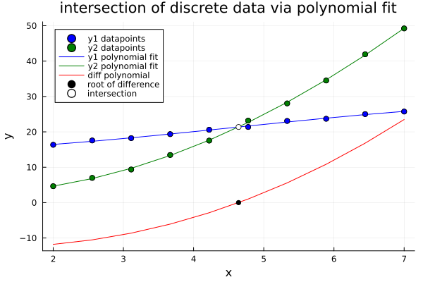
This code block computes polynomial fits, finds the intersection point as a root of the difference polynomial, and plots the results To see how it works and the types it generates, you might want to step through it line by line at the REPL.

y1poly = fit(x,y1, 3)               # make 3rd order polynomial fit to y1 data
y2poly = fit(x,y2, 3)               # same for y2
ydiffpoly = y2poly - y1poly         # compute difference of y2,y1 polynomials

xroots = roots(ydiffpoly)           # find roots of difference polynomial 
j = findall(z -> a ≤ z ≤ b, xroots) # find the indices of the roots with interval (a,b)
xr = xroots[j[1]]                   # select the first root in the interval
yr = y1poly(xr)                     # compute y value at intersection point

scatter(x, y1, label="y1 datapoints", mc=:blue)
scatter!(x, y2, label="y2 datapoints", mc=:green)

plot!(x, y1poly.(x), label="y1 polynomial fit", lc=:blue)
plot!(x, y2poly.(x), label="y2 polynomial fit", lc=:green)
plot!(x, ydiffpoly.(x), label="diff polynomial", lc=:red)

scatter!(x, y1, label="", mc=:blue)
scatter!(x, y2, label="", mc=:green)

scatter!([xr], [ydiffpoly(xr)], label="root of difference", mc=:black)
scatter!([xr], [yr], label="intersection", mc=:white)
plot!(xl="x", yl="y", legend=:topleft)
plot!(title="intersection of discrete data via polynomial fit")

intersection

1 Like

Or, with GMT (intersection point is computed from linear interpolation, I think)

using GMT

f1(x) = 2x + 12;
f2(x) = x^2;

x = range(2, 7, length=10);

y1 = f1.(x);
y2 = f2.(x);

int = gmtspatial(([x y1],[x y2]), intersections=:e);

plot([x y1], limits=(2,7,0,50), marker=:circ, mc=:blue, ms="6p", lw=0.5, lc=:blue)
plot!([x y2], marker=:circ, mc=:green, ms="6p", lw=0.5, lc=:green)
plot!(int, marker=:circ, mc=:red, ms="8p", show=true)

4 Likes

Nice! Though in all honestly I feel the acronym package name GMT hinders discoverability. The name GeneralizedMappingTools.jl would be better for the general public.

EDIT: I see now that GMT.jl is a wrapper for the GMT C library, so the acronym name follows the Julia naming standards.

Yes, and we also have a

  • GMT/MEX, for Matlab
  • pyGMT, for Python
  • GMT.jl for Julia

Not to mention that GMT is a brand with > 30 years, very well known in Geophysics.

1 Like