I am trying to generate a surface plot of the following in Julia. As I’m new, I’m struggling

where \alpha_k are
I’m being able to generate a line plot at a fixed time using the following code:
using Roots,Plots
plotlyjs()

B= 1
Lambda_s=0
f(x) = tan(x) + x ./ (B*(1 .- Lambda_s * x .^2))


N=20
j0=zeros(N)

j0[1]=find_zero(f, 0)

# # print(f.(z0))

for i = 1:length(j0)-1
    j0[i+1] = j0[i] + 2.5;
    j0[i+1] = find_zero(f,j0[i+1]);
end

# print(j0)
# print(f.(j0))
y=f.(j0)

xx = range(0,10,length=100)
yy=f.(xx)
p1=plot(xx,yy, ylims=[-6, 6], title="Eigenvalues" , linewidth=2);
p2=plot(y,xlims=[0, 10],title="Function evaluated at the zeros" , linewidth=2);

p3=plot(j0,title="location of zeros" , linewidth=2);
plot(p1,p2,p3, legend=false)

t=0.2
x=range(0,1,length(j0))


f1= 1 .+ (cos.(j0) .^2 ./(B*(1 .- Lambda_s* j0 .^2))) .+ 2*B*Lambda_s*sin.(j0) .^2
fun= 2*((1 ./ j0) .* (sin.(j0 .* (1 .- x)) ./ f1)) .*exp.(-j0.^2*t)
ff= (1 .+ B*x)/(B .+ 1) .- sum(fun,dims=2)

plot(x,ff, linewidth=2)
Now, I would like to generate a surface plot between t=0 to t=2. Your help will be appreciated.
The above equations are from https://link.springer.com/article/10.1007/s11012-020-01185-3
Write the function just as it’s written in math (simplifying because on phone)
v(y, t) = A*y + sum(x->sin(B*x^2)*exp(-a[x]*t), 1:N)
And then
plot(v, (0, 10), (0, 2); seriestype=:surface)
If the series doesn’t converge nicely (for a small enough N), you’ll need to solve this further, possibly using an analytic framework. But this is how you’d do the plot part.
I tried the following:
# t=0.2
xs=range(0,1,length(j0))
ts=range(0,2,length(j0))
# analytic_sol_func(t,x) =  (x )-(2/pi)*sum([(1/j0[k]* sin(pi*k*(1-x) )*exp(-k^2*pi^2*t ) for k in 1:1:500000])


# f1= 1 .+ (cos.(j0) .^2 ./(B*(1 .- Lambda_s* j0 .^2))) .+ 2*B*Lambda_s*sin.(j0) .^2
# fun= 2*((1 ./ j0) .* (sin.(j0 .* (1 .- x)) ./ f1)) .*exp.(-j0.^2*t)
# ff= (1 .+ B*x)/(B .+ 1) .- sum(fun,dims=2)
# sum([j0[k] for k in 1:1:length(j0)])
# fun= 2*((1 ./ j0) .* (sin.(j0 .* (1 .- x)) ./ (1 .+ (cos.(j0) .^2 ./(B*(1 .- Lambda_s* j0 .^2))) .+ 2*B*Lambda_s*sin.(j0) .^2))) .*exp.(-j0.^2*t)
ff(t,x)= (1 .+ B*x)/(B .+ 1) .- sum([2*((1 ./ j0[k]) .* (sin.(j0[k] .* (1 .- x)) ./ (1 .+ (cos.(j0[k]) .^2 ./(B*(1 .- Lambda_s* j0[k] .^2))) .+ 2*B*Lambda_s*sin.(j0[k]) .^2))).*exp.(-j0[k].^2*t) for k in 1:1:length(j0)])
u_real = reshape([ff(t,x) for t in ts for x in xs], (length(ts),length(xs)))


# surface(ts, xs, ff)
plot(u_real ,ts, xs; seriestype=:surface)
However, it seems like not working. Could you please explain a little more detailed way?
When finding the roots of: tan(x) + x = 0, moving forward by steps of 2.5 is not enough to jump across the singularities. Try:
j0[i+1] = j0[i] + π
For future reference, it’s really difficult to debug something based on “it’s not working” and separate pieces of code that I don’t know how to stitch together. Please read: make it easier to help you.
One thing I see immediately is that the surface plot takes the arguments in the order x, y, Z. But when I run your code, u_real is all NaN, so it’s probably not going to be a very pretty plot.
Here’s a rewrite from the math:
using Roots, Plots
B = 1
Λ_s = 0
N = 20

v(y, t; B, α, Λ_s) = (B*y + 1)/(B + 1) - 2*sum(α_k -> sin(α_k*(1-y))/(α_k*(1 + cos(α_k)^2/(B*(1-Λ_s*α_k^2)) + 2*B*Λ_s*sin(α_k)^2))*exp(-α_k^2*t), α)
f(x) = tan(x) + x/(B*(1-Λ_s*x^2))
α = zeros(N)
for k in 1:N
   α[k] = find_zero(f, (nextfloat(π*(k-3//2)), prevfloat(π*(k-1//2))))
end
plot(α)
plot(range(0,2,100), range(0,1,100), (y,t)->v(y, t; B, α, Λ_s); seriestype=:surface)
Thank you very much for your suggestion. However, when I tried your code, it gives me the following error:
GKS: Rectangle definition is invalid in routine SET_WINDOW
GKS: Rectangle definition is invalid in routine CELLARRAY
invalid range
That’s because the function always returns NaN, because the first term in the summation has 1/α_k = 1/0. Of course analytically we can recognize this as sin(α)/α = 1, but Julia cannot. We need to enforce that the first term is 0, for instance
v(y, t; B, α, Λ_s) = (B*y + 1)/(B + 1) - 2*sum(α_k -> α_k ≈ 0 ? 1 : sin(α_k*(1-y))/(α_k*(1 + cos(α_k)^2/(B*(1-Λ_s*α_k^2)) + 2*B*Λ_s*sin(α_k)^2))*exp(-α_k^2*t), α)

Is that approximately what you expect?
Note that your quoted expression is defined for all α, not just the 20 first positive α starting at 0.0. I don’t know how well this converges.
Thanks for your suggestion.
Avoiding zero gives me a better plot(((k+1/2)*\pi<\alpha[k]<(k+3/2)*\pi)
using Roots, Plots
plotlyjs()
B = 1
Λ_s = 1
N = 100

v(y, t; B, α, Λ_s) = (B*y + 1)/(B + 1) - 2*sum(α_k -> sin(α_k*(1-y))/(α_k*(1 + cos(α_k)^2/(B*(1-Λ_s*α_k^2)) + 2*B*Λ_s*sin(α_k)^2))*exp(-α_k^2*t), α)
# v(y, t; B, α, Λ_s) = (B*y + 1)/(B + 1) - 2*sum(α_k -> α_k ≈ 0 ? 1 : sin(α_k*(1-y))/(α_k*(1 + cos(α_k)^2/(B*(1-Λ_s*α_k^2)) + 2*B*Λ_s*sin(α_k)^2))*exp(-α_k^2*t), α)
f(x) = tan(x) + x/(B*(1-Λ_s*x^2))
α = zeros(N)

for k in 1:N
   α[k] = find_zero(f, (nextfloat(π*(k+3//2)), prevfloat(π*(k+1//2))))

end
# print(α)
plot(range(0,1,100), range(0,6,100), (y,t)->v(y, t; B, α, Λ_s); seriestype=:surface)
The above gives

While the true plot as reported in the article is
Probably some other root-finding method will be needed. I would like to find roots in (0<\alpha[k]<(k+1/2)*\pi). It seems like the above method is not working.
Your limits appear to be in the wrong order, it should be (lowerbound, upperbound). Do you know in which region they find their roots in the paper? Because I don’t know if this converges to the right thing if you only take the start of the positive axis. One strategy that might work is to take every other root negative (for instance, assign \alpha[k] and \alpha[k+1] in the loop, stepping 2:2:2N.
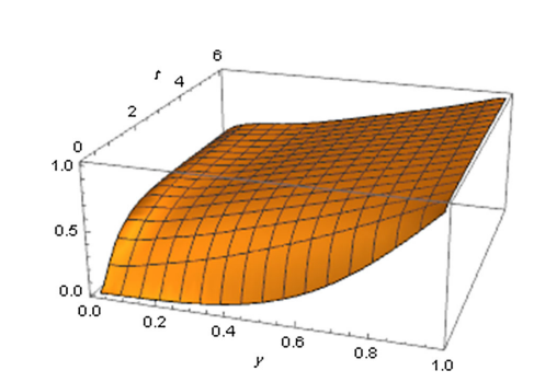
It’s reported in article that, for 0<\frac{1}{\sqrt{\Lambda_s}}\leq \frac{\pi}{2}; \alpha_k satisfy \pi k<\alpha_k<(\pi+0.5)k. Motivated by this, I’ve tried the following:
using Roots, Plots
plotlyjs()
B = 1
Λ_s = 1
N = 100

v(y, t; B, α, Λ_s) = (B*y + 1)/(B + 1) - 2*sum(α_k -> sin(α_k*(1-y))/(α_k*(1 + cos(α_k)^2/(B*(1-Λ_s*α_k^2)) + 2*B*Λ_s*sin(α_k)^2))*exp(-α_k^2*t), α)

f(x) = tan(x) + x/(B*(1-Λ_s*x^2))
α = zeros(N)

for k in 1:N
   α[k] = find_zero(f, (nextfloat(π*(k)), prevfloat(π*(k+1//2))))
end
# print(α)
plot(range(0,1,N), range(0,6,N), (y,t)->v(y, t; B, α, Λ_s); seriestype=:surface)
I’m getting the following plot
It seems pretty reasonable, but not the desired one.
