Quick update:
We are now using uv texture mapping in Makie.jl to visualize “rasters”, which gives an additional 2.5x speedup. If you need this speed, please update your environment.
If you want faster upsampling, look into NNlib. The julia native bilinear upsampling there is parallelized for cpu and gpu and supports 1, 2 & 3D data and is as fast as it can probably get.
Relevant update:
Two job opportunities:
I’m finishing a Masters in Geophysics that is in the geospatial realm (my research is in geodesy). Maybe by the end of my degree I’ll qualify as for being “proficient in high-performance programming languages” because as of now, I’m firmly between novice and adequate. lol
Good luck with the search! ![]()
New discretization and refinement methods, and various other small improvements and fixes.
New MaxLengthDiscretization to discretize geometries into subgeometries of maximum length. This is used in viz of geodesic geometries.
If you create a Segment from two points with LatLon coordinates, and call viz you will see it is “curved”. Below you can see this with random segments:
segs = rand(Segment, 100, crs=LatLon)

viz(segs)
Rings of polygons).
The TriRefinement now supports a predicate function for adaptive refinement. For instance, you can refine all elements with area greater than a given threshold TriRefinement(e -> area(e) > 1km^2).
The georef function now supports a lenunit option besides the crs to specify the length units of some CRS from raw unitless columns.
All Grid subtypes now support CRS (e.g., RectilinearGrid, StructuredGrid, RegularGrid, CartesianGrid). The CartesianGrid is now an alias to a RegularGrid with Cartesian CRS. If you need to convert back and forth between LatLon and Projected coordinates, prefer RegularGrid in your workflows.
We are seeing more and more articles in applied sciences citing the software. Thank you ![]()
This release introduces transiogram functions, which measure the transition probability between categorical values at any given distance along any given direction. Transiograms are used to simulate Markov processes in more than one dimension (e.g. space).
Various models are implemented, including the MatrixExponentialTransiogram model by Carle et al and the PiecewiseLinearTransiogram model by Li et al.
Below is an example where transition probabilities are estimated for 4 categorical values DebrisFlow, Floodplain, Overbank and Channel along the vertical direction.
Another function that was introduced recently is eachvertex, which can be used to iterate over the vertices of a polytope (polygon, segment, etc.) or mesh (e.g. grid) without memory allocation:
for v1 in eachvertex(g1)
  for v2 in eachvertex(g2)
    ...
  end
end
Various other performance optimizations related to eachvertex were implemented to speed things up and reduce the memory usage of specific algorithms.
Appreciate it if you could share your thoughts in our 2025 survey:
Multivariate interpolation with CoKriging that exploits the cross-variable correlation at any lag distance besides the auto-correlation. We support any number of variables, as well as any geostatistical function, including variograms, covariances and transiograms.
CoKriging interpolation is quite useful when a subset of one or more variables are under-sampled, and another subset of densely-sampled variables are linearly correlated to the first subset. The cross-variable correlation can greatly improve the interpolation of the under-sampled variables. Below is an example where we interpolate 5 variables jointly along a well trajectory:
Please reach out in our #geostats.jl channel if you need help setting up multivariate interpolation.
Anisotropic variogram models can now be constructed with ranges and rotation. There is no need to create a MetricBall manually:
GaussianVariogram(ranges = (1, 2, 3), rotation=I)
We took this opportunity to review and optimize the Interpolate and InterpolateNeighbors transforms. Their syntax was simplified to
Interpolate(domain; model=model, ...)
and we no longer support the complex syntax with variable names. This is important now that we have multivariate interpolation routines. If you pass a geotable with N>1 columns to a univariate interpolation model, you will get an assertion error. Please Select(variable) before Interpolate or InterpolateNeighbors in this case.
The variants InterpolateMissing and InterpolateNaN were removed in favor of more explicit pipelines with DropMissing and DropNaN respectively.
We’ve updated the official documentation of the project to include more examples, and cover more undocumented features:
It is far from complete coverage, but already an improvement. We will try to find the time to work on it again during the year, in between our scheduled deliverables.
Full support for multivariate Gaussian simulation, dispatched in the presence of multivariate variogram, covariance or transiogram functions:
# joint covariance model between 2 variables with 0.8 correlation
fun = [1.0 0.8; 0.8 1.0] * SphericalCovariance(range=600)

# Gaussian process with multivariate geostatistical function
proc = GaussianProcess(fun)

# load unstructured mesh from disk
mesh = GeoIO.load("norne.vtu").geometry

# simulate 2 variables jointly over the mesh
real = rand(proc, mesh)
Similar to the previous post about CoKriging, multivariate Gaussian simulation (a.k.a. Gaussian cosimulation) can be useful in contexts where a subset of variables is under-sampled. The main advantage of geostatistical simulation compared to geostatistical interpolation is the reproduction of local features, which are smoothed out by interpolation routines.
New funplot and surfplot functions that generalize and replace old plot recipes for multivariate, anisotropic geostatistical functions:
fun = [1.0 0.8; 0.8 1.0] * SphericalCovariance(ranges=(600,300,200))

funplot(fun)
Alternative simulation methods are chosen much more carefully now based on traits over the type of domain, data and process. If you are using random fields in your work, we highly recommend the update to v0.74.
The rand interface for geospatial stochastic processes is much simpler now:
reals = rand(process, domain, [n]; data=nothing, ...)
It generates n realizations of the stochastic process over the domain. The data is a GeoTable with pre-existing values over the domain or nothing. All pre-existing values are honored by the simulation.
Finally, the varioplot, transioplot and planeplot functions were removed in favor of the more general funplot and surfplot.
I’ve started a FAQ in our official documentation:
If you have suggestions of questions for our FAQ, please let me know or feel free to open a pull request. Happy to review and merge.
New Quenching transform to “smooth” categorical variables obtained from a simulation or learning model. The transform was introduced by Carle & Fogg 1998 to post-process the results of sequential indicator simulation.
In the example below we have the original “raster” with 3 categorical values (left image) and the output of the transform (right image):
The transform accepts any Transiogram function, as well as other parameters to preserve the categorical values at specific locations (e.g., measurements).
As usual, we provide full support for any type of domain, not just grids in a “raster” model, and any type of categorical value, not just integer codes.
New KMedoids clustering transform. The algorithm supports heterogeneous variables (e.g., continuous, categorical, compositional, …) so you can feed GeoTables with all sorts of columns to it. Example below has a single continuous variable and k=3 clusters:
GHC, GSC and SLIC renamed to "label" for consistencyas was removed from these transforms in favor of RenameThe clustering documentation has been updated accordingly:
Quick updates from academia…
GeoStats.jl modules were used in a couple of recent publications:
A benchmark study was published today comparing simple tasks across programming languages, and the potential of these languages for geospatial work:
I would like to take this opportunity to say thank you to all authors who cited our work. A small \cite command in your manuscript makes a huge difference for us ![]()
Various performance improvements with multi-threaded implementations, and various fixes related to floating point issues:
Interpolate and InterpolateNeighbors transforms are multi-threaded now. We are seeing 5x speedups with 8 threads. If you need to perform large-scale 3D Kriging interpolation, that can really make a difference.winding(points, mesh) is multi-threaded now, and therefore our sideof(points, mesh) is benefiting from 2.5x speedups.GrahamScan and consequently convexhull.SutherlandHodgmanClipping and consequently improved performance of intersection of Polygons.RegularSampling methods for simplices, i.e. Triangle and Tetrahedron.simplexify(mesh) is type stable now, leading to downstream performance improvements.Coboundary{P,Q} for GridTopology for any 0<P<Q=D, allowing the lookup of elements sharing edges (for example).intersects predicate with 3D geometries.LambertConic projection and various related EPSG conversions.CarleTransiogram and various other fixes related to transiogram functions.MaxPosterior and ModeFilter transforms to “smooth” categorical variables.MersenneTwister by Xoshiro random number generator.path option in InterpolateNeighbors as it doesn’t change results.These are some of the recent changes I remember by looking into the commit history of all submodules of the project. There are probably more improvements to consider.
We highly recommend updating your environment as usual. Please let us know if you encounter issues with the new release.
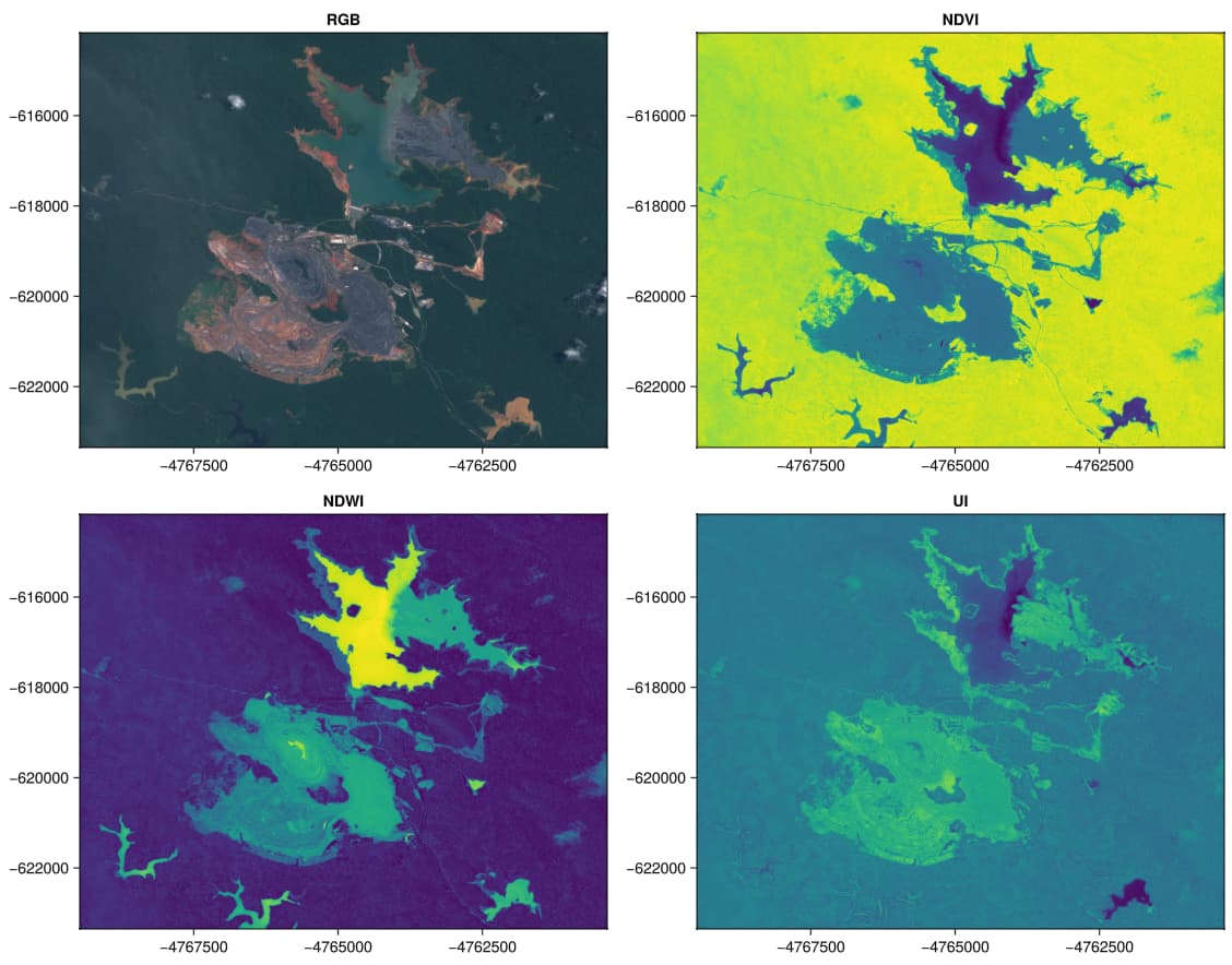
New SpectralIndex transform that makes the awesome SpectralIndices.jl available into a user-friendly interface for GeoTables:
The 247 indices can be listed with the spectralindices function and the bands for a given index can be listed with the spectralbands function.
For example:
julia> spectralbands("NDVI")
2-element Vector{SpectralIndices.Band{String, Int64, Dict{String, SpectralIndices.PlatformBand}}}:
 Band(N: Near-Infrared (NIR))

 Band(R: Red)
The GDSJL book is finally finished ![]()