3D isosurface plotting in Makie

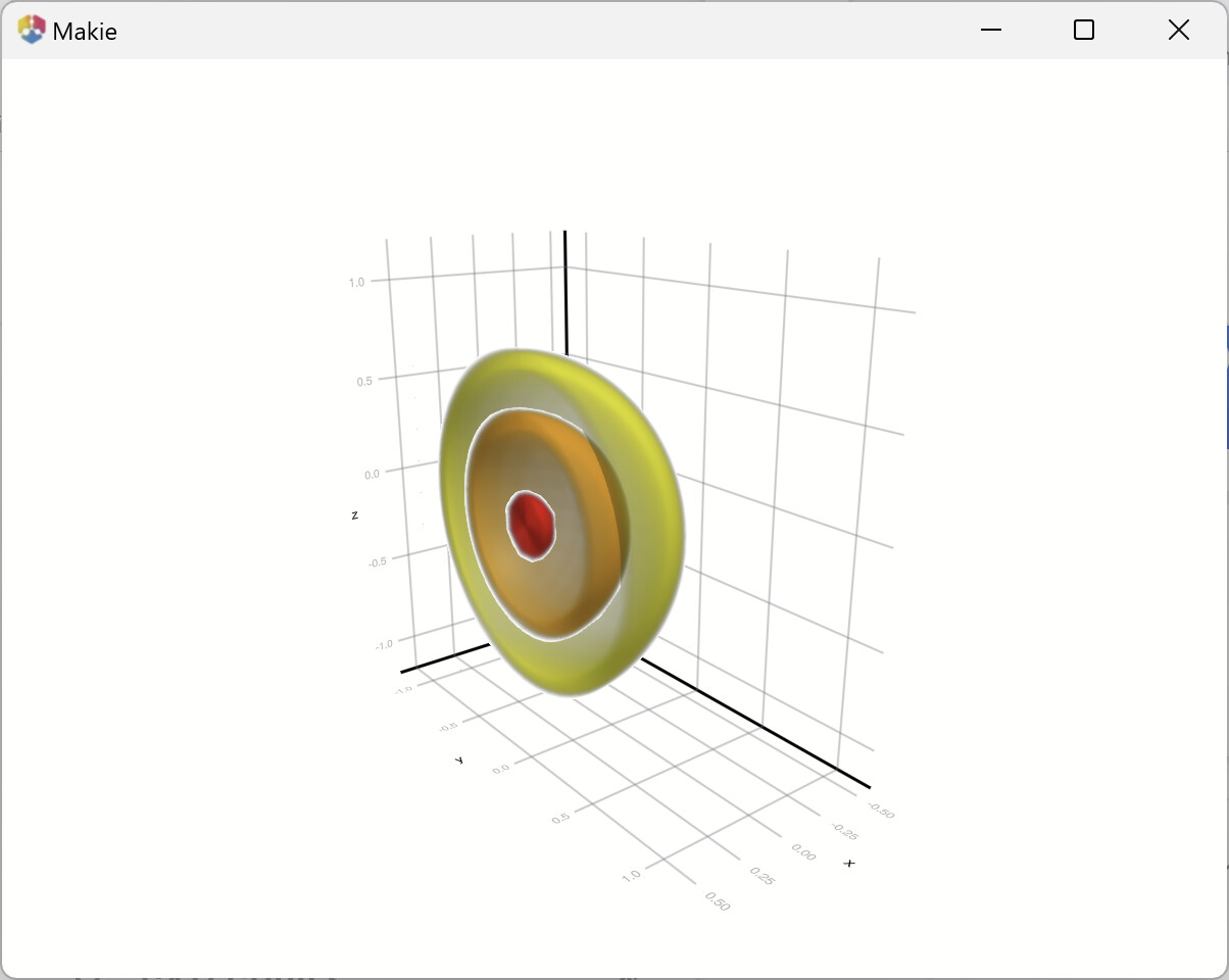
I am using the (semi-)documented contour function for 3D-isosurfaces, cf. volume | Makie, first example.

One cannot define vector of alphas (which would be nice because outer surfaces (shells) “should” be more transparent.

Thus I came up with the following code:

using Statistics, GLMakie, LinearAlgebra

_iscollection(x) = x isa Union{AbstractArray, Tuple, AbstractRange}
# Cycle collections; repeat scalars
_as_iter(x, n) = _iscollection(x) ? Iterators.take(Iterators.cycle(x), n) :
                                   Iterators.repeated(x, n)

function new_iso_contour3d!(
    vol::AbstractArray;
    xs = (1, size(vol, 1)), ys = (1,size(vol, 2)), zs = (1,size(vol, 3)),
    ax = current_axis(),
    levels = quantile(vol, [0.25, 0.50, 0.75]),
    colors = [:yellow, :orange, :red],
    alphas = [0.05, 0.1, 0.2],
)

    lvls = levels isa Number ? (levels, ) : collect(levels)
    L = length(lvls)
    cols = collect(_as_iter(colors, L))
    als  = collect(_as_iter(alphas, L))

    ivx, ivy, ivz = extrema(xs), extrema(ys), extrema(zs)

    for (lev, col, a) in zip(lvls, cols, als)
        contour!(ax, ivx, ivy, ivz, vol;
                 levels=[lev], colormap=cgrad([col, col]), alpha=a)
    end
    nothing
end

r = range(-1, 1, length=20)
vol = [norm([1.2x,y,z]) for x=r, y=r, z=r]
fig = Figure()
ax = LScene(fig[1, 1], scenekw=(show_axis=true,))
new_iso_contour3d!(vol[1:10,:,:]; xs=0.5r, ys=r, zs=r,
    levels=[0.1, 0.5, 0.8], colors=[:red, :orange, :yellow], alphas=[0.2, 0.1, 0.05])

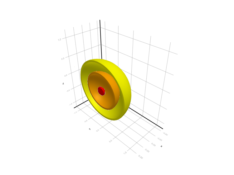
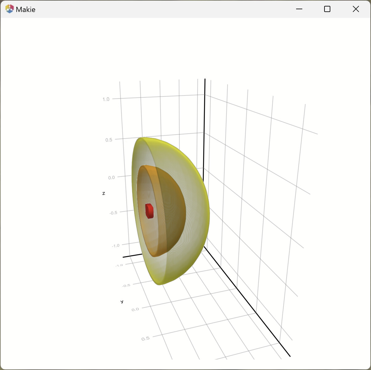
Now, my problem is that the isosurfaces are very thick:

I also tried volume(algorithm=:iso,…) and then a thin isorange, but with smaller alpha the surfaces are really grey. So it would be nice to have control over isorange also from the contour function (?).

I want to plot something, that looks similar to this one below (some years ago with R):

Maybe it is just a matter of the settings in volume(algorithm=:iso,…). Or maybe one can do with surface, but I would not know how exactly. (still new to Julia).

Thanks for any help!

2 Likes

Looking at the source code of contour:

function plot!(plot::Contour{<:Tuple{X, Y, Z, Vol}}) where {X, Y, Z, Vol}
    x, y, z, volume = plot[1:4]
    @extract plot (colormap, levels, linewidth, alpha)
    valuerange = lift(nan_extrema, plot, volume)
    cliprange = map((v, default) -> ifelse(v === automatic, default, v), plot, plot.colorrange, valuerange)
    cmap = lift(plot, colormap, levels, alpha, cliprange, valuerange) do _cmap, l, alpha, cliprange, vrange
        levels = to_levels(l, vrange)
        nlevels = length(levels)
        N = 50 * nlevels

        iso_eps = if haskey(plot, :isorange)
            plot.isorange[]
        else
            nlevels * ((vrange[2] - vrange[1]) / N) # TODO calculate this
        end
        cmap = to_colormap(_cmap)
        v_interval = cliprange[1] .. cliprange[2]
        # resample colormap and make the empty area between iso surfaces transparent
        map(1:N) do i
            i01 = (i - 1) / (N - 1)
            c = Makie.interpolated_getindex(cmap, i01)
            isoval = vrange[1] + (i01 * (vrange[2] - vrange[1]))
            line = reduce(levels, init = false) do v0, level
                isoval in v_interval || return false
                v0 || abs(level - isoval) <= iso_eps
            end
            RGBAf(Colors.color(c), line ? alpha : 0.0)
        end
    end

    return volume!(
        plot, Attributes(plot), x, y, z, volume, alpha = 1.0, # don't apply alpha 2 times
        algorithm = 7, colorrange = cliprange, colormap = cmap
    )
end

I guess the idea (for some reason, it seems quite inefficient) is that we check for ‘all’ values isoval between the minimum and maximum value of volume whether it lies sufficiently close (according to iso_eps) to one of the supplied levels. If so, we draw it using volume! (the source code of which I fail to locate) in a certain colour. (Now, in practice, we cannot check all possible values of course, so we restrict ourselves to a linear grid of N steps. If this grid is too coarse (for a given iso_eps), we might miss a certain level. Makie does not seem to supply any way to directly control N, but by supplying e.g. [0.1, 0.1, 0.1] instead of [0.1] for levels you do triple N. So getting a too coarse grid can be easily circumvented.)

Now suppose you would actually check all possible isovals. Then your shells would have a thickness of 2 * iso_eps. So we want to reduce iso_eps. But as far as I can tell, there’s currently no accessible way to do this. There are some hacky solutions possible though. I’m not fond of any of them as they constitute type piracy, but, hey, they do kind of work.

Overwrite Makie.plot!

Just increase 50 in the definition of N to e.g. 100:

using Makie: nan_extrema, automatic, to_levels, Colors

function Makie.plot!(plot::Contour{<:Tuple{X, Y, Z, Vol}}) where {X, Y, Z, Vol}
    x, y, z, volume = plot[1:4]
    @extract plot (colormap, levels, linewidth, alpha)
    valuerange = lift(nan_extrema, plot, volume)
    cliprange = map((v, default) -> ifelse(v === automatic, default, v), plot, plot.colorrange, valuerange)
    cmap = lift(plot, colormap, levels, alpha, cliprange, valuerange) do _cmap, l, alpha, cliprange, vrange
        levels = to_levels(l, vrange)
        nlevels = length(levels)
        N = 100 * nlevels

        iso_eps = if haskey(plot, :isorange)
            plot.isorange[]
        else
            nlevels * ((vrange[2] - vrange[1]) / N) # TODO calculate this
        end
        cmap = to_colormap(_cmap)
        v_interval = cliprange[1] .. cliprange[2]
        # resample colormap and make the empty area between iso surfaces transparent
        map(1:N) do i
            i01 = (i - 1) / (N - 1)
            c = Makie.interpolated_getindex(cmap, i01)
            isoval = vrange[1] + (i01 * (vrange[2] - vrange[1]))
            line = reduce(levels, init = false) do v0, level
                isoval in v_interval || return false
                v0 || abs(level - isoval) <= iso_eps
            end
            RGBAf(Colors.color(c), line ? alpha : 0.0)
        end
    end

    return volume!(
        plot, Attributes(plot), x, y, z, volume, alpha = 1.0, # don't apply alpha 2 times
        algorithm = 7, colorrange = cliprange, colormap = cmap
    )
end
'Add' isorange

(As a side note, snake case would make clearer we’re not talking about colours or fruits here :slight_smile: .)

function Base.haskey(plot::Contour{<:Tuple{X, Y, Z, Vol}}, symb::Symbol) where {X, Y, Z, Vol}
    symb === :isorange && return true 
    invoke(haskey, Tuple{Plot, Symbol}, plot, symb)
end

function Base.getproperty(plot::Contour{<:Tuple{X, Y, Z, Vol}}, symb::Symbol) where {X, Y, Z, Vol}
    symb == :isorange && return 0.01
    return invoke(Base.getproperty, Tuple{Plot, Symbol}, plot, symb)
end

function new_iso_contour3d!(...)
   (...)
        contour!(...; levels=[lev, lev, lev], ...)
   (...)
end

Results, with alpha=1 for clarity:
(Before, overwriting Makie.plot!, ‘adding’ isorange)


2 Likes

Thanks a lot for these insights! Yes, I could reproduce it with alphas 0.4, 0.2, 0.1 from inside to outside:

The “look and feel” is still different from “real” surfaces I believe, e.g.

Rs = [1, 2, 4]
fig = Figure(size=(1200, 800))
ax = LScene(fig[1, 1], scenekw=(show_axis=true,))
colors=[:red, :orange, :yellow]
alphas=[0.4, 0.2, 0.1]
φs = range(0, π, 20)      # polar angle
θs = range(0, 2π, 40)      # azimuth angle

for i in 1:3
  xs = Rs[i] .* sin.(φs) .* cos.(θs')
  ys = Rs[i] .* sin.(φs) .* sin.(θs')
  zs = Rs[i] .* cos.(φs) .* ones(length(θs), 1)'
  surface!(xs, ys, zs, alpha=alphas[i], color=fill(colors[i], zs |> size))
  wireframe!(xs, ys, zs, color=:black, linewidth=0.5)
end

But in the real case I don’t have the analytical surfaces of course. Also in the rendering of the surface there are strange shading patterns (that’s why I put the wireframe => it is not the surface arangement itself). So probably @eldee solution is the best and I can possibly tweak rendering parameters.

A question I have is: the isorange = 0.01 seems hardwired and can’t be set in a call contour(..., isorange = 0.1, ...) . My Julia insight it not good enough to see how to change it. Actually I thought with haskey and getproperty one could set it.

Don’t remember how the R plot was done, but it was also OpenGL based.

1 Like

There is probably a way to temporarily alter getproperty with the new value, and restore it afterwards. But the easiest option would be to use a global variable (maybe a RefValue):

using Statistics, GLMakie, LinearAlgebra

_iscollection(x) = x isa Union{AbstractArray, Tuple, AbstractRange}
# Cycle collections; repeat scalars
_as_iter(x, n) = _iscollection(x) ? Iterators.take(Iterators.cycle(x), n) :
                                   Iterators.repeated(x, n)

global_isorange::Float64 = 0.01

function Base.haskey(plot::Contour{<:Tuple{X, Y, Z, Vol}}, symb::Symbol) where {X, Y, Z, Vol}
    symb === :isorange && return true 
    invoke(haskey, Tuple{Plot, Symbol}, plot, symb)
end

function Base.getproperty(plot::Contour{<:Tuple{X, Y, Z, Vol}}, symb::Symbol) where {X, Y, Z, Vol}
    symb == :isorange && return global_isorange  # <----
    return invoke(Base.getproperty, Tuple{Plot, Symbol}, plot, symb)
end

function new_iso_contour3d!(
    vol::AbstractArray;
    xs = (1, size(vol, 1)), ys = (1,size(vol, 2)), zs = (1,size(vol, 3)),
    ax = current_axis(),
    levels = quantile(vol, [0.25, 0.50, 0.75]),
    isorange = global_isorange,  # (or calculate like in plot!(::Contour), and/or Vector{Float64})
    levels_factor = 1, 
    colors = [:yellow, :orange, :red],
    alphas = [0.05, 0.1, 0.2],
)

    global global_isorange

    lvls = levels isa Number ? (levels, ) : collect(levels)
    L = length(lvls)
    cols = collect(_as_iter(colors, L))
    als  = collect(_as_iter(alphas, L))

    ivx, ivy, ivz = extrema(xs), extrema(ys), extrema(zs)

    old_isorange = global_isorange
    global_isorange = isorange
    for (lev, col, a) in zip(lvls, cols, als)
        contour!(ax, ivx, ivy, ivz, vol;
                 levels=fill(lev, levels_factor), colormap=cgrad([col, col]), alpha=a, 
                 transparency=true)  # (looks a bit nicer with this set to true)
    end
    global_isorange = old_isorange
    nothing
end

r = range(-1, 1, length=20)
vol = [norm([1.2x,y,z]) for x=r, y=r, z=r]
fig = Figure()
ax = LScene(fig[1, 1], scenekw=(show_axis=true,))
new_iso_contour3d!(vol[1:10,:,:]; xs=0.5r, ys=r, zs=r, ax=ax,
           levels=[0.1, 0.5, 0.8], colors=[:red, :orange, :yellow], isorange=0.03, levels_factor=1, alphas=[0.2, 0.1, 0.05])

ax2 = LScene(fig[1, 2], scenekw=(show_axis=true,))
new_iso_contour3d!(vol[1:10,:,:]; xs=0.5r, ys=r, zs=r, ax=ax2,
           levels=[0.1, 0.5, 0.8], colors=[:red, :orange, :yellow], isorange=0.01, levels_factor=3, alphas=[0.2, 0.1, 0.05])

Building a mesh with MarchingCubes.jl could be an alternative:

using GLMakie
using MarchingCubes
using LinearAlgebra

##

r = range(-1, 1, length=20)
vol = [norm([1.2x,y,z]) for x=r, y=r, z=r]

function contourmesh!(ax, vol, level; kwargs...)
    m = MC(vol)
    march(m, level)
    msh = MarchingCubes.makemesh(Makie.GeometryBasics, m)
    return mesh!(ax, msh; kwargs...)
end

f = Figure()
ax = LScene(f[1, 1])

levels = [0.3, 0.5, 0.8]

for (i, l) in enumerate(levels)
    contourmesh!(ax, vol, l;
        alpha = [1, 0.5, 0.2][i],
        color = [:red, :orange, :yellow][i],
        transparency = true,
    )
end

f

5 Likes

This is spot on! Also the “strange” pattern of surface aren’t there and material properties allow nice customization! Thanks!

We should really add that example to the volume docs! This questions comes up every month or so :wink:

1 Like

I’m always late to these threads but maybe it’s still worth adding some information…

All volume plots do some form of simple ray tracing. For 3D contours a ray steps through the bounding box of the plot, sampling values from the 3D array. These values then sample the colormap using the colorrange to get colors which get blended together. To draw only the requested levels, everything outside of them is transparent in the colormap.

After my pr the colormap density now depends on isorange which effectively controls the thickness of isosurfaces. Hopefully it generates enough color density to avoid skipping isosurfaces now. isorange is also settable again.

I’d argue it’s more realistic. If you look at something like colored glass you will see a darker, more intense color at shallow angles because light passes through more of the material. It’s the same effect here.

transparency = true should help there. The default transparency = false still applies transparency but it’s render order dependent. So it may render all, some or only the front most overlapping triangle.

I didn’t add this, but it shouldn’t be that difficult to add if anyone wants to try. It should just require getting the level index here and something like sv_getindex(alpha, level_index) in the color construction.

1 Like

It still sounds inefficient to me to check uniformly between minimum(volume) and maximum(volume). Why not focus on the regions close to levels? For a fixed ‘budget’ N, I guess it wouldn’t speed up the volume rendering, but you would get more detailed information where it matters (as far as I understand).

We don’t step through the minimum .. maximum range. It’s more like we step through array indices, e.g.

total_color = RGBAf(0,0,0,0)
for i in 1:size(volume, 1)
    value = volume[i, 1, 1]
    total_color += get_color(colormap, colorrange, value)
end

We can’t really shortcut here because we don’t know anything about the volume data. It could be well behaved data where you can do bisection or Newton’s method or something like that. But it could also be repeating or discontinuous or just generally random/not smooth.

Excluding transparent colors from the colormap would be an option, but then we’d need to do something like

for level in levels
    if abs(sample - level) < isorange
        r = level_to_colormap_range(colormap, i)
        value_01 = (sample - level - isorange) / (2 * isorange)
        color = get_interpolated_color(view(colormap, r), value_01)
        return color
    end
end

instead of just

get_interpolated_color(colormap, (sample - colorrange[1]) / (colorrange[2] - colorrange[1])

We’d likely just get worse performance for a lower memory overhead. Quality would probably be more or less the same because we still work with the same isorange and number of samples.

Could you link to the volume/volume! implementation? That would presumably make things clearer. (Also more generally, how would one go about finding such code? Makie seems very difficult to navigate.)

You’re probably referring to volume! here, but I was talking about contour! (plot!(::Contour)):

valuerange = lift(nan_extrema, plot, volume)
cmap = lift(..., valuerange) do ..., vrange
    map(1:N) do i
        i01 = (i - 1) / (N - 1)
        isoval = vrange[1] + (i01 * (vrange[2] - vrange[1]))
    end
end

I think you misunderstood what I was talking about with the non-uniform idea. As an example, suppose you have data in [0, 1] and are looking for the isosurface for value 0.5 using N = 4. Then currently the cmap could be something like

  • [0, 0.33) → transparent
  • [0.33, 0.67) → blue
  • [0.67, 1] → transparent.

But alternatively, you could use e.g.

  • [0, 0.45) → transparent
  • [0.45, 0.55) → blue
  • [0.55, 1] → transparent.

I would expect this to result in better-defined boundaries, which is what you would want for a contour plot. The volume rendering itself would not change.

3D contours are volume plots. They end up running this shader function

That code got updated in 0.24.6

That controls the thickness of the isosurface which is set by isorange. The attribute was broken from 0.24.0 to 0.24.5 though. In 0.24.6 you can set it again and it has an effect on the generated colormap:

using Colors, Makie
f,a,p = contour(rand(10,10,10), isorange = 0.1, levels = [0.5])
count(c -> alpha(c) != 0.0, p.computed_colormap[]) # 14 visible colors
length(p.computed_colormap[]) # 100 total

f,a,p = contour(rand(10,10,10), isorange = 0.01, levels = [0.5])
count(c -> alpha(c) != 0.0, p.computed_colormap[]) # 5 visible colors
length(p.computed_colormap[]) # 260 total

If you’re talking about the fuzziness/blur on the … surface of the surfaces, e.g. the left and right edges here


then that comes from the shader interpolating between an opaque color and a transparent one. That can sort of be reduced by increasing the total number of colors in the colormap, because then you go through the interpolation faster. If you want to get rid off it completely you’d have to change the shader algorithm though.

1 Like

Indeed, but it still works uniformly, going from the (padded colorrange) minimum and maximum of the volume data:

map!(
    plot,
    [..., :padded_colorrange, :computed_isorange...],
    :computed_colormap
) do ..., (min, max), isorange, ...
    N = ceil(Int, 2.5 * (max - min) / isorange)
    ...
    return map(1:N) do i
        isoval = min + (i - 1) / (N - 1) * (max - min)
        ...
    end
end

Using isorange you can control N and hence the thickness. But I still feel like it makes more sense to cluster the isovals around the levels values (when levels is a Vector), instead of taking them uniformly. Going back to the example, contrast a uniform ‘cmap’ for N = 10

  • [0,0.11) → transparent
  • [0.11, 0.22) → transparent
  • [0.22, 0.33) → transparent
  • [0.33, 0.44) → transparent
  • [0.44, 0.56) → blue
  • [0.56, 0.67) → transparent
  • [0.67, 0.78) → transparent
  • [0.78, 0.89) → transparent
  • [0.89, 1.) → transparent

(where 90% of the intervals are transparent, i.e. non-informative), with a non-uniform equivalent with N = 4

  • [0,0.44) → transparent
  • [0.44, 0.56) → blue
  • [0.56, 0.1) → transparent

Conversely, I would expect that the non-uniform version for N = 10, which splits up the ‘blue’ interval, is somehow more detailed. But I’d need a bit more time to think about how the cmap is actually used. Maybe this would only be useful if you decrease the opacity in the ‘blue’ interval farther away from the levels values or something like that.

It’s of course also entirely possible that in practice this all does not matter as increasing N comes at a negligible cost.

Right, this is what I meant with the get_interpolated_colormap comments. With this

you just need to transform values to indices to get the appropriate color. In GLSL you can use a 0..1 value as an index, so it’s just texture(colormap, (sample - 0) / (1 - 0)).

With this your colormap is [:transparent, :blue, :transparent]. To get :blue only in the appropriate interval you now need to explicitly check if (0.44 <= sample < 0.56); return colormap[2].

Yea I think that’s probably the case. The cost of making a 1000 element array in Julia isn’t particularly large and it’s probably not something that updates frequently either. The GPU upload only happens when the data changes and the up-front cost of uploading something is quite significant afaik. So adding a couple KB might not matter much.

1 Like