Unable to use lagrange to solve 2 varable functions in modeling toolkit

	@parameters x_1 x_2
	@variables u 

   eqs = [ 0 ~ u - (x_1+2)*(x_2+1), 130 ~ 4*x_1+6*x_2]

@named sys = NonlinearSystem(eqs, [x_1, x_2],[])

prob = NonlinearProblem(structural_simplify(sys),[x_1=>1.0,x_2=>1.0,u=>max])

generates an error, saying that there is no equation for x_1

I am not yet perfectly familiar with ModelingToolkit, but just looking at your code, it seems that you are mixing the roles of a parameter and a variable. You declare x_1 and x_2 as parameters but then you treat them as variables (as if you wanted to solve the problem with respect to them). Isn’t this the cause of the problem? Have a look at Modeling Nonlinear Systems · ModelingToolkit.jl, they enter variables and parameters separately in NonlinearSystem() and NonlinearProblem().

4 Likes

Here is a working example:

using ModelingToolkit, NonlinearSolve

@variables x_1 x_2
@parameters u = 1.


eqs = [ 0 ~ u - (x_1+2)*(x_2+1), 130 ~ 4*x_1+6*x_2]

@named sys = NonlinearSystem(
    eqs,
    [x_1, x_2],
    [u],
    defaults = [
        x_1 => 1,
        x_2 => (130 - 4*x_1)/6
        ]
)

prob = NonlinearProblem(structural_simplify(sys), [])
solve(prob, NewtonRaphson())
1 Like

Thanks, I was confused on variables snd parameters, and thus cleared it up. Only thing is that I don’t know u , but I want yo maximize u.

You might want to check GalacticOptim and OptimizationProblem in ModelingToolkit.

I’ll reiterate my suggestion to use JuMP instead:

do i replace prob with:

prob = OptimizationProblem(structural_simplify(sys),[x_1=>1.0,x_2=>1.0,u=>1.0])

I want to learn both, so that I can compare them. I’ve done this in JuMP and that is defiantly a valid option.

I am still not sure I understand what you are after. You write

But then if x_1 and x_2 are known/given/fixed, and you impose the constraint 0 ~ u - (x_1+2)*(x_2+1), and there is not freedom left for you to do any optimization whatsoever. Your u is just given by the equation. Nothing to maximize here.

u(x_1,x_2)=(x_1+2)*(x_2+1) u is meant to be a function of x_1 and x_2

I see. Only now I get it. To summarize, the full description of the problem is therefore this:

maximize (x_1+2)*(x_2+1)

subject to 4*x_1+6*x_2 = 130

Concerning your attempted solving of this problem using ModelingToolkit, it appears to me that NonlinearSystem() is just an equation solver (it cannot do maximization) and the OptimizationSystem() cannot accept constraints. This is at least what I get from the docs, I hope I have not overlooked anything.

1 Like

It sounds like I’m better off using JuMP then.

1 Like

By the way, if the particular structure of the problem is typical of your needs, this is a QP problem (a quadratic cost function and linear equality constraints). As such it can be solved without a general optimization package just by using a solver for linear equations (look the KKT matrix up if you are not familiar with it, for example here).

Here comes a code

# Parameterization of the quadratic cost function 1/2 x'Qx + r'x + c
Q = [0.0 1.0; 1.0 0.0]
r = [1.0, 2.0]
c = 2.0

# Parameterization of the linear constraint Ax = b
A = [4.0 6.0]
b = 130

# KKT linear system
K = [hcat(Q,A'); hcat(A, 0)]
d = vcat(-r,b)
y = K\d

The maximum is at

julia> xopt = y[1:2]
2-element Vector{Float64}:
 16.0
 11.0

That this is truly a maximum can be verified by checking negativity of the projected Hessian, which in this case can be computed using

julia> Z = nullspace(A);

julia> Z'*Q*Z
1×1 Matrix{Float64}:
 -0.923076923076923

We are lucky here because the Hessian of the uncostrained cost function is actually indefinite (the matrix Q has one positive and one negative eigval) and the unconstrained problem is unbounded. But for the contstrained problem we have a (unique and bounded) maximum.
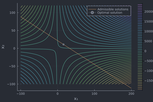
Finally, some plots

# Plotting the cost function, the constraint and the optimal solution
using Plots

f(x₁,x₂) = (x₁+2)*(x₂+1)

x₁ = range(-100.0,200.0,length=500)
x₂ = range(-100.0,120.0,length=500)

plot(x₁,x₂,f,st=:surface,xlabel="x₁",ylabel="x₂",zlabel="f(x₁,x₂)")

fcn

contour(x₁,x₂,f,xlabel="x₁",ylabel="x₂",levels=50)
x₂sol(x₁) = (130.0-4*x₁)/6
plot!(x₁,x₂sol,label="Admissible solutions")
plot!([y[1]],[y[2]],markershape=:circle,label="Optimal solution")

contour

4 Likes

What package are you using?

Package for what? I used nothing but the backslash for solving the linear equations (well, the code should have started with using LinearAlgebra because I also computed nullspace).

This makes sense, I’m not sure I know enough about linear algebra. I’m going through an Econ text now, and can find stuff about matrices in an earlier chapter. Are the matrices used Hessian matrices?

I get that Q is the null matirx, and A is a matrix of prices, but what do r and c mean?

I got the matrices by manually rewriting your function u(x_1,x_2) = (x_1+2)(x_2+1) to be maximized into the vector form

f(\boldsymbol x) = \frac{1}{2}\boldsymbol x^\top \mathbf Q \boldsymbol x + \mathbf r^\top\boldsymbol x + c.

This conversion of format was nearly instinctive and automatic for me as soon as I observed that it is a quadratic function. Having it then in this compact vector format opens a reservoir of results and tools.

Note that as you can read in the code, \mathbf Q = \begin{bmatrix}0&1\\1&0\end{bmatrix}, which is surely not a null matrix. I also call it Hessian because in this case of a quadratic function this matrix is all that is left after differentiating the function twice with respect to the vector \boldsymbol x (and Hessian matrix is nothing else than a matrix composed of second derivatives).

3 Likes

What matrix is Q, I can’t remember the name, but I remember it being the simplest matrix, where each variable is simplified to one.

No idea what you mean :grinning:

I’m getting an idea of how Jacobians and Hessians work, I think that I’ll need to go over these topics.

One thing I noticed in your plots, and mine when I recreated them, is that the scale is weird. I was able to change the parameters of x1 and x2, but then I added the linear portion, when below zero,and with the ideal marked, it became the same as yours.