Hi folks, ![]()
Been doing a lot of work with the great SciML ecosystem and building more familiarity with its offerings.
I am struggling with an ODE that I am trying to model. Here is the equation:
\frac{dI}{dt} = a \cdot \frac{B}{k + B} \cdot S - r \cdot I
Which I wrote in the function:
I(a, k, r, S, B, I) = (a * S) * (B / (k + B)) - r * I
As a, k, and r are constants, I replaced them in my formulation as follows:
I(S, B, I) = (1 * S) * (B / (10e6 + B)) - 0.2 * I
For this ODE, I had the initial values for S, B, and I:
initial_values =
    [
     H - 1, # S(0)
     0, # B(0)
     1, # I(0)
    ]
Where H is a population count comes from me looping over a set number of population counts. I read up on how to pass multiple parameters to my ODE using DifferentialEquations.jl and came up with a final function formulation that looked like this:
I(I, p, t) = ((a_1 * p[1]) * (p[2] / (k_1 + p[2]))) - (r_1 * p[3])
My full code is as follows:
# Setting up labeling of the figure
fig = Figure(fontsize = 24);
ax = Axis(fig[1, 1],
          title = L"Plot of $I$",
          xlabel = L"t",
          ylabel = L"Population Size"
);

# Time interval from $0$ to $20$ days
tspan = (0, 20)

# Total human populations
populations = [5000, 6000, 7000, 8000, 9000, 10000]

# ODE I am evaluating
I(I, p, t) = ((a_1 * p[1]) * (p[2] / (k_1 + p[2]))) - (r_1 * p[3])

# Looping through different population sizes
for H in populations

initial_values =
    [
     H - 1, # S(0)
     0, # B(0)
     1, # I(0)
    ]

    # Set-up ODE
    prob = ODEProblem(I, 1, tspan, initial_values)

    # Use Tsit5 solver for non-stiff ODEs
    sol = solve(prob, Tsit5(), reltol = 1e-8, abstol = 1e-8)

    lines!(ax, sol.t, sol.u, label = L"H = $H")
end

# Show plot
fig
However, the figure output (below) doesn’t seem to be matching what I expect (next figure).

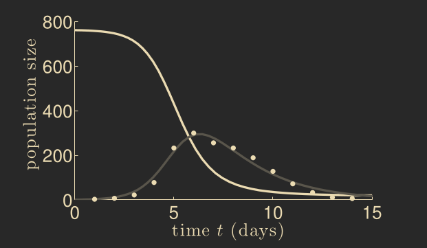
Even though the values aren’t exactly the same (they shouldn’t be since I am looking at different populations), they are all coming out to the same line and I don’t see any behavior variation that I would expect like in the second figure.
Could anyone point out to me what I may be doing wrong with my ODEProblem set-up? I was thinking I am somehow screwing up my implementation but unsure where.
Thanks!
~ tcp ![]()
P.S. For full transparency, this is part of a homework assignment but I am allowed collaboration.