Solving a Shifted Linear System of 2 Symmetric Positive Semi Definite (SPSD) Matrices

I have the following linear system:

\left( \boldsymbol{A} + \lambda \boldsymbol{C} \right) \boldsymbol{x} = \boldsymbol{A}^{T} \boldsymbol{b}

Where \boldsymbol{A}, \boldsymbol{C} \in \mathcal{S}_{+}^{n} are Symmetric Positive Semi Definte (SPSD) Matrices.

I need to solve the system for various \lambda > 0 values.
Beside using LDL Decomposition on \boldsymbol{A} + \lambda \boldsymbol{C} or “Hot Iteration”, is there an efficient way to solve this?
Similar to the case \boldsymbol{C} = \boldsymbol{I}?

I can’t assume the matrices are similar.

Remark: Once could think on the above as the Normal Equations of a Tikhonov Regularized Least Squares:

\arg \min_{\boldsymbol{x}} \frac{1}{2} {\left\| \boldsymbol{D} \boldsymbol{x} - \boldsymbol{b} \right\|}_{2}^{2} + \frac{\lambda}{2} {\left\| \boldsymbol{E} \boldsymbol{x} \right\|}_{2}^{2}

Where \boldsymbol{A} = \boldsymbol{D}^{T} \boldsymbol{D} and \boldsymbol{C} = \boldsymbol{E}^{T} \boldsymbol{E}.
If there a specialized way to solve this for various \lambda values without the squared condition number, it would be even better.

There are a few options, but it is a harder problem and those options aren’t as nice as for A-\lambda I. I’m assuming that you aren’t trying to exploit sparsity. You could try treating this as a symmetric semi-definite generalized eigenvalue problem to simultaneously diagonalize A and C with a common congruence formed from generalized eigenvectors. The stability of that is not perfect, however. The eigenvector matrix can be ill-conditioned and if C is semidefinite instead of positive definite, you are not even guaranteed a complete set of eigenvectors.

What I have done before is to just to give up on exploiting symmetry. If you compute a Hessenberg-triangular form of A and C:

Q^T A Z = H, \qquad Q^T B Z = R

where H is upper Hessenberg and R is upper triangular. Q and Z are orthogonal. Your problem transforms to

(H + \lambda R) \mathbf{y} = Q^T A^T \mathbf{b}

where \mathbf{y} = Z^T \mathbf{x}. Each choice of \lambda then gives a Hessenberg system to solve, which is more efficient. The LAPACK routine for Hessenberg-triangular reduction is xGGHRD. Unfortunately, there doesn’t appear to be an existing Julia interface to that routine. But it probably isn’t too hard to write. I’ve found the existing Julia interfaces not that hard to follow as a template for accessing other LAPACK routines. Although, to be honest, last time I had a problem like this, I was too lazy to do that and just used schur(A,C), so it had to run the full QZ algorithm. It was mostly something I was doing for some test code and it slowed down the tests, but I could live with that.

There is a symmetry preserving reduction that will use a congruence to make A tridiagonal and C diagonal, which is a lot closer to the A-\lambda I case. But you give up on orthogonality of the congruence. There is a description in this paper. I’d trust the non-symmetric approach more for stability.

I don’t know what options there are that avoid condition squaring for the regularized least squares problem. I have actually thought a little about that before, but didn’t come up with anything and I haven’t seen anything published. I’m not sure that it’s reasonable to expect to do this. Using orthogonal transformations would automatically preserve symmetry when you form D^T D and E^T E and symmetry and orthogonality don’t seem to go together for this type of reduction. So you can probably do something, but I wouldn’t expect it to be fully based on orthogonal transformations and there might be stability concerns.

2 Likes

One option is to first Cholesky-factor C = U^T U, let y = U x, then rewrite the system as:

(\underbrace{U^{-T} A U^{-1}}_{B} + \lambda I) y = U^{-T} A^T b = c

Note that the matrix B is still SPSD. Note also that, as usual, you don’t actually invert any matrices: you compute B via triangular solves B = U' \ A / U.

Once you have it in this form, you can call hessenberg(Hermitian(B)) to factorize B into Q H Q^T, where H is symmetric tridiagonal. The advantage of this is that you can then do shifted solves without repeating the factorization, since B + \lambda I = Q (H + \lambda I) Q^T.

(Diagonalizing B into eigenvectors would also accomplish this, but is more expensive. On the other hand, diagonalization results in a faster solve step, so it depends on how many \lambda you need to solve with.)

Moreover, the Hessenberg factorization objects in Julia have efficient specialized support for shifted solves, for exactly this sort of application.

In short, you can do something like:

# pre-processing
U = cholesky(C).U # UpperTriangular
B = Hermitian(U' \ A / U)
c = U' \ (A'b)
F = hessenberg(B) # tridiagonal

# solve for each λ
λ = 0.1234
y = (F + λ*I) \ c
x = U \ y

# check:
@show x ≈ (A + λ*C) \ (A'b)  # should print "true"

Note that F + \lambda*I is actually lazy — it doesn’t even allocate a new matrix. And you can do the y and x solves in-place too, if you have pre-allocated vectors x and y:

ldiv!(y, F + λ*I, c)
ldiv!(x, U, y)

Usually if you are doing Tikhonov regularization, the resulting system should be well-conditioned, no?

If it’s ill-conditioned, you could equivalently solve the ordinary least-squares problem

\min_x \left\Vert \begin{pmatrix} D \\ \sqrt{\lambda} E \end{pmatrix} x - \begin{pmatrix} b \\ 0 \end{pmatrix} \right\Vert_2

by QR as usual (\ in Julia), but I’m not sure if there is a way to re-use calculations for multiple \lambda in that case.

2 Likes

Indeed. I meant mostly in case solving it directly and not using the Normal Equations can yield something even better.

The only issue with your solution is to handle the case the matrices \boldsymbol{A} and \boldsymbol{C} are not SPD and hence the Cholesky factorization is not feasible.
Unless you mean \boldsymbol{U} is derived using the Eigen Decomposition with the root of the diagonal matrix. But the then the assumption about the triangular won’t hold.

Could it be done with LDLt?

You mean C could be singular?

The whole point of Tikhonov is to choose an E such that C = E^T E is positive-definite, as that is what makes the regularization A + \lambda C work. That is, you should choose an E matrix with independent columns (full column rank). Otherwise your problem need not even have a unique answer, and you need to re-think what you are even doing.

As long as C is SPD and \lambda > 0, then it doesn’t matter if A is only SPSD.

If A and C could be arbitrary SPSD matrices, then you haven’t provided enough information to specify an answer. e.g. what x do you want to get if A = C = zeros(m,m)? Or is your problem somehow such that A + \lambda C is always nonsingular/SPD?

PS. If at least one of either A or C is SPD, you are fine: if C is singular but A is SPD, simply swap the two matrices by solving (C + \mu A)x = \mu A^T b where \mu = \lambda^{-1}, and apply my approach by Cholesky-factoring A instead of C.

I agree that in the usual case things are as you described.
Yet in my case, both are SPSD, namely in some cases both are indeed singular.

For the case one is SPD I was aware of the trick you mentioned, though with the Eigen Decomposition instead of the Hessenberg (Probably saw you posting it somewhere else in the forum).

My own reasons for wanting decompositions of this type was looking at error bounds for the symmetric semidefinite generalized eigenvalue problem and comparing a more stable algorithm to the standard Cholesky approach when C is ill-conditioned (and for the algorithm I was working on, possibly singular). It was an intermediate step in using inverse iteration to compute condition number estimates of A-\lambda B where \lambda is an approximate generalized eigenvalue to determine if \lambda had been computed in a way that gives a small backward error. I really needed to stick purely to orthogonal transformations to preserve the singular values of A-\lambda B for the comparison to be meaningful.

I did take the part about C being singular to heart, but it is certainly odd to see a linear system of this type where C is singular. It would be nice to know where it comes from.

1 Like

In my actual problem, in one of the steps I optimize something like:

\arg \min_{\boldsymbol{x}} \boldsymbol{x}^{T} \boldsymbol{E}_{1} \hat{\boldsymbol{A}} \boldsymbol{E}_{1} \boldsymbol{x} + \lambda \boldsymbol{x}^{T} \boldsymbol{E}_{2} \hat{\boldsymbol{C}} \boldsymbol{E}_{2}\boldsymbol{x}

Where the matrices \boldsymbol{E}_{1}, \boldsymbol{E}_{2} generate a weighted subset of \boldsymbol{x}. They might have zero columns. More than that, it might share same idnices of such columns.
So the above \boldsymbol{A} = \boldsymbol{E}_{1}^{T} \hat{\boldsymbol{A}} \boldsymbol{E}_{1}, \; \boldsymbol{C} = \boldsymbol{E}_{2}^{T} \hat{\boldsymbol{C}} \boldsymbol{E}_{2}.

By the nature of the matrices, they are not guaranteed to be SPD.

I can do some cherry picking of the elements, but the issue is this is a single step of multiple steps and it is nicer to keep this structure even if it means the matrices are SPSD and not SPD.

I just thought a similar trick to the one above can be employed in such case as well.

I have wanted to try this for a while and I did try setting up an interface to the Hessenberg-triangular form from LAPACK with the following:

using LinearAlgebra
using LinearAlgebra: checksquare, libblastrampoline
using LinearAlgebra.LAPACK: BlasInt, @chkvalidparam, @blasfunc, chkstride1, chklapackerror
using Base: require_one_based_indexing

for (gghd3, elty) in
    ((:dgghd3_,:Float64),
     (:sgghd3_,:Float32))
    @eval begin
        function gghd3!(jobq::AbstractChar, jobz::AbstractChar,
                        A::AbstractMatrix{$elty}, B::AbstractMatrix{$elty})
            require_one_based_indexing(A, B)
            @chkvalidparam 1 jobq ('N', 'I')
            @chkvalidparam 2 jobz ('N', 'I')
            chkstride1(A, B)
            n, m = checksquare(A, B)
            ilo = 1
            ihi = n
            if n != m
                throw(DimensionMismatch(
                    lazy"dimensions of A, ($n,$n), and B, ($m,$m), must match"))
            end
            ldq = jobq == 'I' ? max(1, n) : 1
            q = similar(A, $elty, ldq, n)
            ldz = jobz == 'I' ? max(1, n) : 1
            z = similar(A, $elty, ldz, n)
            work = Vector{$elty}(undef, 1)
            lwork = BlasInt(-1)
            info = Ref{BlasInt}()
            for i = 1:2  # first call returns lwork as work[1]
                ccall((@blasfunc($gghd3), libblastrampoline), Cvoid,
                      (Ref{UInt8}, Ref{UInt8}, #compq, compz
                       Ref{BlasInt}, Ref{BlasInt}, Ref{BlasInt},  # n, ilo, ihi
                       Ptr{$elty}, Ref{BlasInt}, Ptr{$elty}, # A, lda, B
                       Ref{BlasInt}, Ptr{$elty}, Ref{BlasInt}, # ldb, Q, ldq
                       Ptr{$elty}, Ref{BlasInt}, Ptr{$elty}, # Z, ldz, work
                       Ref{BlasInt}, Ref{BlasInt}, # lwork, info
                       Clong, Clong, Clong),
                      jobq, jobz,
                      n, ilo, ihi, A, max(1,stride(A, 2)), B,
                      max(1,stride(B, 2)), q, ldq, z,
                      ldz, work, lwork, info, 1, 1, 1)
                chklapackerror(info[])
                if i == 1
                    lwork = BlasInt(real(work[1]))
                    resize!(work, lwork)
                end
            end
            UpperHessenberg(A), UpperTriangular(B),
            q[1:(jobq == 'I' ? n : 0),:], z[1:(jobz == 'I' ? n : 0),:]
        end
    end
end


function hess_triangular_form(A,B)
    Q1, R = qr(B)
    Ta, Tb, Q, Z = gghd3!('I', 'I', Q1'*A, R)
    return Ta, Tb, Q1*Q, Z
end

This can be used to solve the system with something like

using LinearAlgebra

n=100
A = randn(n,n)
B = randn(n,n)
Ta, Tb, Q, Z = hess_triangular_form(A,B)

@show opnorm(A-Q*Ta*Z', Inf)
@show opnorm(B-Q*Tb*Z', Inf)

b = randn(n)
y = Q'*A'*copy(b)
λ = 7.0
ldiv!(UpperHessenberg(Ta + λ * Tb), y)
x = Z*y
@show norm((A + λ * B) * x - A'*b)

which gives output:

opnorm(A - Q * Ta * Z', Inf) = 2.580362139237291e-13
opnorm(B - Q * Tb * Z', Inf) = 2.2466750682070824e-13
norm((A + λ * B) * x - A' * b) = 7.710934030831613e-13

Solving should be O(n^2) once the Hessenberg-triangular form is computed with cost O(n^3). The built-in schur(A,B) in Julia goes a bit further than Hessenberg-triangular form and makes A quasi-triangular (with at most 2\times 2 blocks on the diagonal) and B triangular. It can be used in the same way, since it’s a more structured Hessenberg-triangular form. I thought the basic Hessenberg triangular form would be a substantial performance improvement over going to the full Schur form, but again with random A and B, for n=1000 I get

julia> @benchmark hess_triangular_form(A,B)
BenchmarkTools.Trial: 2 samples with 1 evaluation per sample.
 Range (min … max):  3.845 s …   3.933 s  ┊ GC (min … max): 0.04% … 0.00%
 Time  (median):     3.889 s              ┊ GC (median):    0.02%
 Time  (mean ± σ):   3.889 s ± 62.658 ms  ┊ GC (mean ± σ):  0.02% ± 0.03%

and

julia> @benchmark schur(A,B)
BenchmarkTools.Trial: 2 samples with 1 evaluation per sample.
 Range (min … max):  4.608 s …   4.658 s  ┊ GC (min … max): 0.00% … 0.02%
 Time  (median):     4.633 s              ┊ GC (median):    0.01%
 Time  (mean ± σ):   4.633 s ± 35.495 ms  ┊ GC (mean ± σ):  0.01% ± 0.01%

(Note in the above numbers, the computer I’m running this on is ancient.)
So it appears to be pretty marginal. Profiling suggests that hess_triangular_form is spending most of its time in the ccall, so I don’t think the allocations and the simple set-up of the problem is taking much time. I’m a bit surprised, but maybe the Hessenberg-triangular form is a larger percentage of the schur run time than I thought it was. I was expecting half or less.

2 Likes

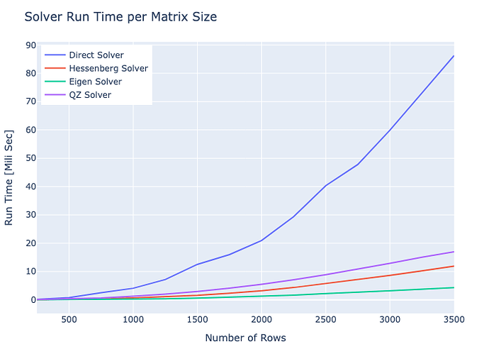
I benchmarked the 3 approaches:

  • Direct: Using Cholesky on the original formulation.
  • Hessenberg: As above.
  • Eigen: Using eigen decomposition on \boldsymbol{B} in @stevengj 's answer.

In each I tried to optimize away allocations.
I didn’t measure the decomposition time (Which might be important for small cases).
This is for example the Hessenberg function:

function SolveHessenberg( mH :: H, α :: T, vD :: Vector{T}, mU :: UT, vX :: Vector{T}, vY :: Vector{T} ) where {T <: AbstractFloat, H <: Hessenberg, UT <: UpperTriangular}

    ldiv!(vY, mH + α * I, vD);
    ldiv!(vX, mU, vY);

    return vX;

end

On my AMD Ryzen 9 7940HS, Julia 1.10.10 with OpenBLAs on Windows 11, those are the results:

The code is available in SolveShiftedLinearSysetm.jl.

It is interesting yet I was aware of those methods. They don’t fit my use case (A loop in an ADMM solver).
I’m still looking for optimization which can handle the case the matrices \boldsymbol{A}, \boldsymbol{C} are SPSD yet not SPD (Namely they have a zero eigenvalue).

@mstewart , If you can build a function in the format above, I’d be happy to test it in this use case.

OK, I think I missed it for some reason, but I can do as following:

  • Decompose using the LDL Decomposition: \boldsymbol{C} = \boldsymbol{L} \boldsymbol{D} \boldsymbol{L}^{T}.
  • Multiply both ends of the equation by \boldsymbol{L}^{-1} to yield \boldsymbol{L}^{-1} \left( \boldsymbol{A} + \lambda \boldsymbol{L} \boldsymbol{D} \boldsymbol{L}^{T} \right) \boldsymbol{L}^{-T} \boldsymbol{L}^{T} \boldsymbol{x} = \boldsymbol{L}^{-1} \boldsymbol{b}.
  • Define \boldsymbol{E} = \boldsymbol{L}^{-1} \boldsymbol{A} \boldsymbol{L}^{-T}, \boldsymbol{y} = \boldsymbol{L}^{T} \boldsymbol{x} and \boldsymbol{f} = \boldsymbol{L}^{-1} \boldsymbol{b} will yield \left( \boldsymbol{E} + \lambda \boldsymbol{D} \right) \boldsymbol{y} = \boldsymbol{f} where \boldsymbol{E} is SPSD.
  • The case where \boldsymbol{D} is all positive is solved easily (See above or Shifted Krylov methods).
  • The motivation for this case is some values are zeros. In this case the system should be decomposed into zeros and non zeros (Block System). It can be tuned into a form of a smaller system with all positive diagonal system.

For more complexity one can use Eigen Decomposition on \boldsymbol{C} and go through the same logic with Orthogonal Matrices instead of Triangular.

Solving Shifted System with Non Negative Diagonal Matrix

This section describes how to solve the following case:

\left( \boldsymbol{E} + \lambda \boldsymbol{D} \right) \boldsymbol{y} = \boldsymbol{f}

Where {D}_{i, i} \geq 0 and \boldsymbol{E} \in \mathcal{S}_{+}^{n}.

Since some of the last elements are zeros \boldsymbol{D} = \operatorname{Diag} \left( \begin{bmatrix} \boldsymbol{d}_{s} \\ \boldsymbol{d}_{z} \end{bmatrix} \right) where {{d}_{s}}_{i} > 0. One can reformulate the problem accordingly:

\left( \begin{bmatrix} \boldsymbol{E}_{SS} & \boldsymbol{E}_{SZ} \\ \boldsymbol{E}_{SZ} & \boldsymbol{E}_{ZZ} \end{bmatrix} + \alpha \operatorname{Diag} \left( \begin{bmatrix} \boldsymbol{d}_{s} \\ \boldsymbol{d}_{z} \end{bmatrix} \right) \right) \begin{bmatrix} \boldsymbol{y}_{s} \\ \boldsymbol{y}_{z} \end{bmatrix} = \begin{bmatrix} \boldsymbol{f}_{s} \\ \boldsymbol{f}_{z} \end{bmatrix}

The system can be decomposed into 2 systems:

\begin{align*} \left( \boldsymbol{E}_{SS} + \lambda \operatorname{Diag} \left( \boldsymbol{d}_{s} \right) \right) \boldsymbol{y}_{s} + \boldsymbol{E}_{SZ} \boldsymbol{y}_{z} & = \boldsymbol{f}_{s} \\ \boldsymbol{E}_{SZ} \boldsymbol{y}_{s} + \boldsymbol{E}_{ZZ} \boldsymbol{y}_{z} & = \boldsymbol{f}_{z} \end{align*}

Define \boldsymbol{u} = \boldsymbol{E}_{ZZ}^{-1} \boldsymbol{f}_{z}, \boldsymbol{v} = \boldsymbol{f}_{s} - \boldsymbol{E}_{SZ} \boldsymbol{u}, \; \boldsymbol{P} = \boldsymbol{E}_{ZZ}^{-1} \boldsymbol{E}_{ZS}, \; \boldsymbol{Q} = \boldsymbol{E}_{SS} - \boldsymbol{E}_{SZ} \boldsymbol{P} and form the system:

\left( \boldsymbol{Q} + \lambda \operatorname{Diag} \left( \boldsymbol{d}_{s} \right) \right) \boldsymbol{y}_{s} = \boldsymbol{v}

Which is a Shifted System of SPSD matrix + Positive Diagonal which can be solved as above.
To recover \boldsymbol{y}_{z} use \boldsymbol{y}_{z} = \boldsymbol{u} - \boldsymbol{P} \boldsymbol{y}_{s}

That doesn’t quite work. Starting with

(E + \lambda D) \boldsymbol{y} = \boldsymbol{f}

you have

(QSQ^T + \lambda D) \boldsymbol{y} = \boldsymbol{f}
Q(S + \lambda Q^T D Q) Q^T \boldsymbol{y} = \boldsymbol{f}

so that

\boldsymbol{y} = Q (S + \lambda Q^T D Q)^{-1} Q^T \boldsymbol{f}.

What fails is that Q^T D Q won’t be diagonal.

You’re right. I was sloppy. For some reason I remembered I had already done something like that for the case of a shifted system of SPSD + Diagonal.

Update: I did remembered correctly that I handled it once. Just not the way above. I updated the message to reflect what I did.

I guess I will just use the Pivoted Cholesky path.

Here is what I had in mind, in a somewhat similar format to your function:

using LinearAlgebra

function SolveHessenbergTriangular!( Ha :: H, Tc :: UT,
                                     Q :: M, Z :: M, λ :: T,
                                     vD :: Vector{T}, vX :: Vector{T},
                                     vY :: Vector{T},
                                     work :: H) where {T <: AbstractFloat,
                                                       H <: UpperHessenberg,
                                                       UT <: UpperTriangular,
                                                       M <: AbstractMatrix}

    mul!(vX, Q', vD)
    work .= Ha .+ λ .* Tc
    ldiv!(vY, work, vX)
    mul!(vX, Z, vY)
    return vX
end

# Make A and C semidefinite
n=100
r = 52
A = randn(n,r)
A = A * A'
C = randn(n,r)
C = C * C'

# workspaces
vD = randn(n)
work = UpperHessenberg(randn(n,n))
vX = zeros(n)
vY = zeros(n)

Ha, Tc, Q, Z = schur(A,C)

λ = 7.0

SolveHessenbergTriangular!(UpperHessenberg(Ha), UpperTriangular(Tc),
                           Q, Z, λ, vD, vX, vY, work)

@show norm((A + λ * C) * vX - vD)

The decomposition is probably much slower than the other options and I would expect the per system time to be a bit slower as well. The only reason to do this is if C is singular or ill-conditioned enough that you are worried about stability. You can make the factorization marginally faster with the LAPACK stuff I posted earlier, but it’s not a huge improvement.

2 Likes

Note that the benchmarking here also depends on the balance between the O(m^3) startup cost and the O(m) or O(m^2) cost of each \lambda's solve. How many shifted solves do you typically need?

If you need \ll m solves, I suspect that only the startup time matters.

Indeed. As I mentioned in the post, I did not account the overhead which can be significant in small number of iterations.

I use it as an inner loop in ADMM solver. So probably the number of iterations is 100-500.

Yet the challenge is dealing with Semi Definite matrices. I think I sketched something above. Yet I am not sure how robust it is.
It seems that @mstewart 's solution is the most stable.

Edit, mostly deleted what I wrote: I wrote a bunch of nonsense here because I focused on the possibility of D_z potentially containing some nonzero elements, when the point was that it should presumably be a zero block.

Yes. I do think this works if E_{zz} is nonsingular. But I do not believe that can be guaranteed. So this is not fully general.

The Fix-Heiberger reduction starts in this way but then makes a further rank decision on E_{zz} and further refines the partition of E and D to deal with the possibility that E_{zz} is singular. It probably would work somewhat robustly in this case, but it’s a more complicated algorithm and I don’t think it ever made it into LAPACK.

1 Like

How big are the matrices?

1 Like

I guess they are in the range of 50-5000.
From my analysis:

  • the gain for large matrices (1000 and above) is ranging 20-100 [Mili Sec] per iteration.
  • It means 50 iterations benefit at least 1 Sec for Pre Processing. Since I use ADMM it probably means 2-5 Sec for Pre Processing.

Since in most cases the pre processing will be faster than gain, I’d assume using the Eigen / Hessenberg makes sense. The only caveat is what are the implications of Pivoted Cholesky on SPSD matrices which dure to numerical issues will have small negative eigen values.
This is why I thought it would be better to have LDL Decomposition and clip the negative values.

Any thoughts on that?

I added the QZ Decomposition based solution as described by @mstewart .
I also added a run time benchmark for the Pre Process step per method,
The results on my Apple M2 Max PowerBook with Julia 1.11.6 with OpenBLAS is:

The remaining question is how robust will be a Pivoted Cholesky approach as it seems to be the best balance if it works.

I updated the code Gist: SolveShiftedLinearSysetm.jl.