Solve a routine economics PDE from an HJB w/ ModelingToolkit

Consider a routine continuous time optimization problem from economics:
V(t,a_{t}) := \max \int_{\tau=t}^{\tau = T} e^{-\rho (\tau -t)} u(c_{\tau})d\tau \text{ s.t. }
\dot{a}_{t} = y + ra_{t} - c_{t},
a_{0} \text{ given, } a_{T}=0.
Assume y & r are constants and u(c)=\frac{c^{1-\gamma}}{1-\gamma}.

The problem has a known closed form solution:
image
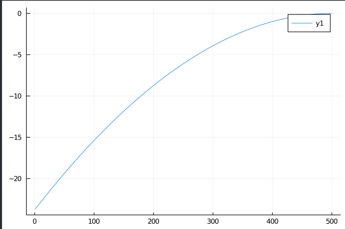
Here I plot V(0,a_{t}) and V(t,1):

To solve this using the HJB approach requires solving a PDE:
\left[\begin{array}{l} \rho V(t,a_{t}) = \frac{c_{t}^{1-\gamma}}{1-\gamma} + V_{a}(t,a_{t})\times \left(y + ra_{t} - c_{t} \right) + V_{t}(t,a_{t}) \\ c(t,a_{t}) = (V_{a}(t,a_{t}))^{-\frac{1}{\gamma}} \\ V(T,a_{T}) = 0 \end{array} \right]

Iā€™m trying to solve it w/ ModelingToolkit.jl, but itā€™s taking forever & not converging.

using NeuralPDE, Flux, ModelingToolkit, GalacticOptim, Optim, DiffEqFlux
using Plots

@parameters t a Īø
@variables V(..)
@derivatives Da'~a
@derivatives Dt'~t

#
u(c,Ī³)= (c^(1.0 -Ī³))/(1.0 -Ī³);
Ī³  = 2.00; Ļ = 0.01; r = 0.01; y = 0.00; T = 5.0;
Ļ‰  = r - (r-Ļ)/Ī³;
# Closed form solution.
VS(t,a;y=y,r=r,Ī³=Ī³,Ļ‰=Ļ‰,T=T)=
    u(a+(y/r), Ī³) * ( (1.0 - exp(-Ļ‰*(T-t))) / Ļ‰ )^Ī³;
# if r=Ļ
CS(t,a;y=y,r=r,Ī³=Ī³,Ļ‰=Ļ‰,T=T, a0=1) = (r*a0)/(1.0 - exp(-r*T) )
AS(t,a;y=y,r=r,Ī³=Ī³,Ļ‰=Ļ‰,T=T, a0=1) =
    (a0)/(1.0 - exp(-r*T) ) +
    a0*(1.0 - 1.0/(1.0 - exp(-r*T) ) ) * exp(r*t);

plot(  VS.(0.0,0.01:.01:5.0) )
plot( VS.(0.0:.01:5.0,1.0) )

#
v  = V(t,a,Īø);
va = max(eps(), Da(V(t,a,Īø)) );
vt = Dt(V(t,a,Īø));
c  = (va)^(-1.0/Ī³);
#uc = u(c,Ī³)
uc = (va^(1.0 - 1.0/Ī³) )/(1.0 - Ī³);
# HJB
eq  = Ļ*v ~ uc + va*(y + r*a - c) + vt;

# Boundary conditions
bcs = [V(T,a,Īø) ~ 0.0] #0.f0
# Space and time domains
domains = [t āˆˆ IntervalDomain(0.0,5.0),
           a āˆˆ IntervalDomain(0.0,5.0)]
# Discretization
dx = 0.1

# Neural network
dim = 2 # number of dimensions
chain = FastChain(FastDense(dim,16,Flux.Ļƒ),FastDense(16,16,Flux.Ļƒ),FastDense(16,1))
discretization = PhysicsInformedNN(dx,chain)

pde_system = PDESystem(eq,bcs,domains,[t,a],[V])
prob = discretize(pde_system,discretization)

cb = function (p,l)
    println("Current loss is: $l")
    return false
end

res = GalacticOptim.solve(prob, Flux.ADAM(); cb = cb, maxiters=10)
res = GalacticOptim.solve(prob, Optim.BFGS(); cb = cb, maxiters=10)

#
phi = discretization.phi
ts,as = [domain.domain.lower:dx/10:domain.domain.upper for domain in domains]
u_predict = reshape(
    [first(phi([t,a],res.minimizer)) for t in ts for a in as],
    (length(ts),length(as))
    )

# plot V(t=0,a)  #u_predict[1,:]
plot(as, u_predict[1,:])  
# plot V(t, a=0.01)
plot(ts, u_predict[:,1])
  1. it takes forever & is not accurate
  2. originally I plugged in the exact equation but got an error
ERROR: DomainError with -0.05701087375174788:
Exponentiation yielding a complex result requires a complex argument.
Replace x^y with (x+0im)^y, Complex(x)^y, or similar.
  1. the issue is the pde has terms like V_{a}(t,a_{t})^{-\frac{1}{\gamma}} and we have numerical problems related to dividing by zero or taking the root of negative numbers.
    We would like to use the prior knowledge that V_{a}>0.
  2. following a suggestion @matthieu , I tried max(eps(), va)^(-1/Ī³)
    No more domain error, but it takes forever & is not accurate.

Note: if \gamma >1 the trivial solution V(t,a_{t})=0 also satisfies the PDE.
It can be avoided w/ a bequest motiveā€¦

dont you need a boundary condition?

@rveltz yes.
Itā€™s V(T,a_{T})=0 for the unknown function V(t,a_{t}).
In the code bcs = [V(T,a,Īø) ~ 0.0].

That said, most successful attempts to solve HJBs use viscocity solutionsā€¦

Does the numerical algo implements the ideas behind viscosity solutions?

1 Like

Youā€™ll have to ask the people who created the packageā€¦
I know the code uses a new gen of methods that solves pdes w/ Neural Networks.
Those methods have been shown to be very successful at solving high-dim HJB equations.
I also know that the package is still in itā€™s early phase.

To clarify, Iā€™m trained as an economist (my undergrad was in math but no PDEs).
That means I know how to set up a problem that boils down to a pde, but I count on experts to make solvers where I can plug in my PDE (do a little tuning) and voila.

Iā€™ve used Mathematica & a few others. I wanna switch to Julia.

I am not quite sure about this, but in any case for the above problem a spectral method (eg Chebyshev polynomials) should be very accurate and super-fast (either limit the domain to a relevant interval [recommended], or transform [-1,1] to \mathbb{R}).

A change of variables can improve on this even further.

I think I just mentioned this somewhere else too. If you know the solution is positive, then force it.

FastChain(FastDense(dim,16,Flux.Ļƒ),FastDense(16,16,Flux.Ļƒ),FastDense(16,1),(x,p)->x^2)

Thatā€™s a neural network that is a universal approximator for positive functions.

1 Like

Sorry I wasnā€™t clear.
The solution to the PDE V(t,a_{t}) is not positive in general (see plots in my original post above).

I know that c>0, and since V_{a}(t,a_{t})=c^{-\gamma} and \gamma>0, we will have V_{a}(t,a_{t})>0.

I donā€™t know how to incorporate this information (V_{a}(t,a_{t})>0).

So youā€™re looking for a monotonic neural network?

Yes, in this case, I know that the unknown function V(t,a_{t}) is monotonically increasing in both itā€™s arguments. (is that what youā€™re asking?)

The PDE that needs to be solved:
\left[\begin{array}{l} \rho V(t,a_{t}) = \frac{ (V_{a} )^{\frac{\gamma-1}{\gamma}}}{1-\gamma} + V_{a}(t,a_{t})\times \left(y + ra_{t} - (V_{a})^{-\frac{1}{\gamma}} \right) + V_{t}(t,a_{t}) \\ V(T,a_{T}) = 0 \end{array} \right]

In my example \gamma =2
\left[\begin{array}{l} \rho V(t,a_{t}) = -(V_{a} )^{\frac{1}{2}} + V_{a}(t,a_{t})\times \left(y + ra_{t} - (V_{a})^{-\frac{1}{2}} \right) + V_{t}(t,a_{t}) \\ V(T,a_{T}) = 0 \end{array} \right]
The problem is the term (V_{a})^{-\frac{1}{2}} .
I just want it to know that V_a >0 so it doesnā€™t worry about dividing by zero or taking roots of negative numbersā€¦

Yes. So youā€™d be looking for a monotonic neural network. I donā€™t exactly know of an architecture that gives that, but thatā€™s what youā€™re looking for.

2 Likes

It doesnā€™t really work to discretize this way in general, though it can sometimes in specific circumstances. The issue is that control problems have a very peculiar backwards/forwards structure, which leads to specialized discretization schemes where some parts of the equation are discreitized forwards and others backwards. Then things converge to the viscosity solution. Not to say that other approaches canā€™t work, but the convergence of these things is very complicatedā€¦ You canā€™t just throw equations at an optimizer.

With spectral-style methods (or just using a neural network with a function) rather than finite difference methods you probably can get away just minimizing residuals with all of your equations with some neural network approximation, but I can say with experience that they are very finicky for HJBE problems with a control. Boundary conditions are trickyā€¦ If you want to do transition dynamics without a control choice, in which case it is kind of like a HJBE without much of an ā€œHā€, then you can use simpler discretizations.

For something along the lines of what you are describing I think it is a little premature in terms of the theory. For one thing, you are describing a finite time-horizon setup, which is of limited usefulness to most economists, but mostly it is that there is a vast literature on this due to the peculiarities of these equations. Also, I think it very unlikely that neural networks will beat the standard algorithms (e.g. codes - HACT - Benjamin Moll - University of Princeton ) for this dimensionality.

3 Likes

Not sure if this helps or confuses. I have some code for monotonic regression. Might have a bug or something, doubtful itā€™s differentiable. Pretty sure itā€™s an active set optimization - but itā€™s been a while since Iā€™ve lookedā€¦
https://github.com/caseykneale/ChemometricsTools.jl/blob/cf53867beb273bffc6deb22d8d060a09c68278ae/src/RegressionModels.jl#L273

My experience is the opposite: they are fast, especially if you get a good initial guess (from the previous set of parameters if you are estimating, or some trick like consistent future approximations), and very accurate. They are also simple to implement (basically working through Miranda-Fackler makes you a black-belt HJB ninja).

In contrast, treating a HJBE like a PDE and discretizing is something that I never manage to implement reliably. The problem is not that I cannot get it working for one set of parameters, but when I am estimating a model it has to work for all sorts of wacky parameters all the time.

1 Like

Certainly they are amazing in discrete time, and for stationary problems in continuous time (with simple enough boundary conditions). My issues might have all come down to boundary conditions.

But if you have non-stationary problems (i.e. the terminal T in the quetsion he asked) then I am not sure if Miranda-Fackler has examples for bellmans/stochastic control? Do you go spectral in time? I am not sure what they would suggest for PDEs rather than the stationary ODEs.

But @Albert_Zevelev he is 100% right to start with Miranda and Fackler for this. In some ways, I think it is best to think of the neural network stuff as more similar to the collocation approaches than finite-differencesā€¦ but there may be different ways to set it up.

But donā€™t forget that one of the requirements for these sorts of spectral or collocation based approaches is taking the derivative of the function you are approximating with. With a polynomial basis this is easy (especially using compecon) but with neural networks you would need to get the derivative. No problem, but then you also need to differentiate that to get the gradients to minimize the loss. So you need to do reverse over forward diff or something. Not impossible, but this would take tinkering and the convergence properties will end up being original research, were I to guess.

2 Likes

Personally I donā€™t have a lot of experience with these models, but yes, I have seen people do this.

But of course ā€” thatā€™s what always happens. It will consume 97% of the time spent on the project, and end up in the appendix in a very shortened form :wink:

1 Like

Do you have example of code where this is done?

About this I am not sure. New and rigorous convergence proofs have a more prominent place in the numerical analysis literature. (Whether in this case such a proof would indeed be new, I cannot judge. It is not my field.) If you can demonstrate convergence and apply it to an interesting class of problems, it is even better, of course.

1 Like

That may be, but unfortunately general equilibrium problems in economics are quite badly behaved, so most methods are ad hoc (ā€œwe did that, and it workedā€). Also, from reading what people use in physics, the applications are about 2 decades behind.

1 Like

I have seen it at a conference a couple of years ago, tried to find it but couldnā€™t, sorry. But it would not help with Julia code either I guess (this was years ago).

But I see no reason why approximating V(t, a) with Chebyshev polynomials (tensored, or Smolyak if you want to be really fancy) shouldnā€™t just work. I would just deal with the possible sign problem with \max(V_a, 0), or a smooth maximum with small scale to get an initial solution near the correct one.