I have one of those, but not in a compact code.
From here: GitHub - m3g/CKP
I have one of those, but not in a compact code.
From here: GitHub - m3g/CKP
@LaurentPlagne posted this beautiful example: 
See Plot a circle with a given radius with Plots.jl. I don’t know if he has published the code for it though.
] activate .
instantiate
This is some of my favorite Julia code.
Thank you for the comment ![]()
Unfortunately I don’t think that it can fit the 7 lines example list (>1000 SLOC)…
We use this example to show how to structure a not-too-small project (PkgSkeleton, types, modules, sub-modules, tests, export, dependencies, multiple dispatch, profile, //isme …) in our Julia training lectures.
Although I enjoy reading the examples in this thread, I would second @Tamas_Papp saying that Julia’s power is more strongly demonstrated through slightly larger examples.
We must take some time to refactor the package from its training material form and publish it : now I have an extra motivation to see if a Julia wizard could compact it significantly ![]()
Side note: Love the color scheme. What are you using for it?
I think seven lines of code is excellent. It showcases what Julia can do, and hopefully shows how Jukia can express scientific notation or equations in a compact way.
However one small pleading from me. Let’s now go down the road of Obfuscated Perl. Back in the day when Perl was a dominant language for Web programming, and many other things, there were a lot of smart people involved. Still are probably! There were regular ‘Obfuscated Perl’ competitions.
Also the whitespace as code stuff (where you translate code into …err… meaningful whitespace ) etc.
I know I am being like the Grinch but IMHO these did the language no good
Don’t get me wrong - there is nothing bad about using a language feature but please, please explain what it does so other people can learn.
I recently started using SatelliteToolbox.jl, so here is my submission. This code calculates the location (latitude, longitude, altitude) of the ISS “right now”. The readability suffers a bit trying to stick to seven, but it’s not too bad. This is based off of the example here (see the link for full details).
using Dates, SatelliteToolbox
# Download data for ISS
download("https://celestrak.com/NORAD/elements/stations.txt", joinpath(pwd(), "space_stations.txt"))
# Initialize the orbit propagator
orbp = init_orbit_propagator(Val(:sgp4), read_tle("space_stations.txt")[1])
# Get the current time (Julian date)
rightnow = DatetoJD(now())
# Propogate the orbit to "right now"
o, r_teme, v_teme = propagate_to_epoch!(orbp, rightnow)
# Get the position (radians, radians, meters)
lat, lon, h = ECEFtoGeodetic(rECItoECEF(TEME(), ITRF(), rightnow, get_iers_eop())*r_teme)
# Nice print out after conversions
println("Current location of the ISS: $(rad2deg(lat))°  $(rad2deg(lon))°  $(h/1000) km")
@mihalybaci Is Santa tracking data available on 24 December?
![]()
Not sure, I poked around here a bit, and didn’t see anything for Santa. But this site gets its data from NORAD, and they’re the ones that do the Santa tracking, so it could be hidden in a file somewhere.
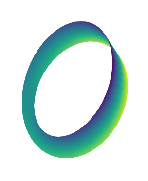
Möbius discovered the one-sided non-orientable strip in 1858 while serving as the chair of astronomy at the University of Leipzig. The concept inspired mathematicians in the development of the field of topology as well as artists like M.C. Escher.
Fifteen lines of Julia were required to compute and plot the Mobius strip and a moving normal vector, which changes color after each 2π revolution. This exceeds the limit but someone might be able to compress it further.
(PS: edited code for better readability. Without sleep, the last for loop could be written as a comprehension too)
using Makie, ForwardDiff, LinearAlgebra
const FDd = ForwardDiff.derivative

M(u,v) = ((r + v/2*cos(u/2))*cos(u), (r + v/2*cos(u/2))*sin(u), v/2*sin(u/2))
∂M∂u(u,v) = [FDd(u->M(u,v)[1],u), FDd(u->M(u,v)[2],u), FDd(u->M(u,v)[3],u)]
∂M∂v(u,v) = [FDd(v->M(u,v)[1],v), FDd(v->M(u,v)[2],v), FDd(v->M(u,v)[3],v)]

r = 1.0; w = 0.5; m = 90; clr = (:cyan,:red,:cyan,:red,:cyan)
u = range(0, 8π, length = 4m); v = range(-w, w, length = 3)

N = [ -cross(∂M∂u(ui, 0.0), ∂M∂v(ui, 0.0))[j] for ui in u, j in 1:3 ]
N = N ./ sqrt.(sum(abs2,N,dims=2));  N = vec.(Point3f0.(N[:,1],N[:,2],N[:,3]))
xs, ys, zs = [[p[i] for p in M.(u, v')] for i in 1:3]
P0 = vec.(Point3f0.(xs[:,2], ys[:,2], zs[:,2]))

surface(xs[1:m+1,:], ys[1:m+1,:], zs[1:m+1,:], backgroundcolor=:black)
for i in 1:4m
    sleep(0.01); k = 1 + i÷(m+0.5);
    arrows!([P0[i]],[N[i]],lengthscale=0.3,arrowsize=0.05,arrowcolor=clr[k],linecolor=clr[k])
end
Instead of compressing it further - I’d be more interested to see it broken out to be more readable :). Awesome plot though!
For what it is worth, Makie’s ˋbandˋ function actually makes 2d bands in 3d space… comes in handy for your Möbius strips:
t = 0:0.1:2pi+0.1
lower = [Point3f0(.2cos(3s),0.0, 0.0) .+ (1 + 0.2sin(3s))*Point3f0(0, cos(s), sin(s)) for s in t]
upper = [Point3f0(-.2cos(3s),0.0, 0.0) .+ (1 - 0.2sin(3s)).*Point3f0(0, cos(s), sin(s)) for s in t]
band(lower, upper, color = [1.0:length(t)÷2; length(t)÷2:-1:1.0; length(t)÷2:-1:1.0; 1.0:length(t)÷2])
Would you mind sharing the code for that normal vector?
The orientability depends on the parity of the number of twists.
That depends on how many times the band is twisted before it is glued back together.
Depends whether it is an even or an odd number of turns ![]() , factor
, factor 3s corresponds to 6 turns which is even, here is s/2 one turn
lower = [Point3f0(.2cos(s/2),0.0, 0.0) .+ (1 + 0.2sin(s/2))*Point3f0(0, cos(s), sin(s)) for s in t]
upper = [Point3f0(-.2cos(s/2),0.0, 0.0) .+ (1 - 0.2sin(s/2)).*Point3f0(0, cos(s), sin(s)) for s in t]
band(lower, upper, color = [1.0:length(t); length(t):-1:1.0], show_axis=false)
Not orientable. I also do a little trick with the colouring.
@dpsanders, the code is the same as in the Mobius strip further above (using the partial derivatives and cross product). Just changed M(u,v) consistently with @mschauer’s strip definition:
M(u,v) = (v/2*cos(3u), (r + v/2*sin(3u))*cos(u), (r + v/2*sin(3u))*sin(u)) # other strip by @mschauer
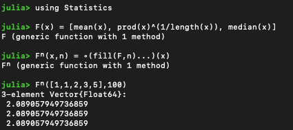
Very nice, I hope you’ll forgive me stealing this in a math.stackexchange comment at real analysis - For what values does the geothmetic meandian converge? - Mathematics Stack Exchange ![]()