I adapted your script to work with an LTI that is closer to the problem I am trying to solve. So I moved to ControlSystems.jl and c2d.
Since you are obviously the expert on all of these packages could you perhaps take a look at this script in case you spot anything that could be done better? I would really appreciate it 
(it is self-contained so it should be possible to just run it)
using Pkg
cd(@__DIR__)
Pkg.activate(".")
using LowLevelParticleFilters
using LowLevelParticleFilters: SimpleMvNormal
using StaticArrays
using LinearAlgebra
using Random
using Plots
using StatsPlots
using Optimization
using ControlSystems
using Distributions
using OptimizationOptimJL
# basic 3-state LTI with 3 inputs and 2 outputs
"""
thermal_dynamics(p)
Create continuous-time state-space system for thermal model.
Arguments:
- p: Parameters [C_i, C_e, C_h, R_ia, R_ie, R_ea, R_ih, A_e, A_w]
Returns: Continuous-time StateSpace system
"""
function thermal_dynamics(p)
C_i, C_e, C_h, R_ia, R_ie, R_ea, R_ih, A_e, A_w = p
A = SA[
(-1/R_ia+-1/R_ie+-1/R_ih)/C_i 1/(C_i*R_ie) 1/(C_i*R_ih);
1/(C_e*R_ie) (-1/R_ea+-1/R_ie)/C_e 0;
1/(C_h*R_ih) 0 -1/(C_h*R_ih)
]
B = SA[
1/(C_i*R_ia) 0 A_w/C_i;
1/(C_e*R_ea) 0 A_e/C_e;
0 1/C_h 0
]
C = SA[
1.0 0.0 0.0;
0.0 0.0 1.0
]
D = @SArray zeros(2, 3)
return ss(A, B, C, D)
end
# true parameter values [C_i, C_e, C_h, R_ia, R_ie, R_ea, R_ih, A_e, A_w]
p_true = [12.0, 45.0, 0.3, 3.0, 1.5, 70.0, 5.0, 1.2, 8.0]
# simulation settings
Ts = 0.25 # Sample time [hours]
n_days = 4 # Number of days to simulate
T = Int(floor(n_days * 24 / Ts)) # Number of time steps
t = 0:Ts:(T-1)*Ts
# we have three measured disturbances to consider:
# u[1]: (measured) ambient temperature
# u[2]: (measured) heat supplied
# u[3]: (measured) solar radiation
# ambient temperature [°C]
u_1 = 10 .+ 8 * sin.(2π * (t .- 6) / 24)
# prbs input for heat supplied
Random.seed!(42)
u_2 = zeros(T)
for k in 1:T
if rand() < 0.01
u_2[k] = 10.0 * (rand() - 0.5)
elseif k > 1
u_2[k] = u_2[k-1]
end
end
# heat supplied (non-negative) [kW]
u_2 = max.(u_2, 0.0)
# solar radiation [kW/m²]
u_3 = 0.4 .* max.(sin.(2π * (t .- 6) / 24), 0.0)
# noise covariances
R1 = Diagonal(SA[0.01, 0.01, 0.01])
R2 = Diagonal(SA[0.5, 1.0])
# discrete-time system
sys_c = thermal_dynamics(p_true)
sys_d = c2d(sys_c, Ts, :tustin)
"""
measurement(x, u, p, t)
Measurement function: we observe T_i (indoor temperature) and T_h (heater temperature)
State: x = [T_i, T_e, T_h]
Output: y = [T_i, T_h]
"""
measurement(x, u, p, t) = SA[x[1], x[3]]
# generate true trajectory using lsim
x0 = SA[20.0, 15.0, 22.0] # initial state
# u needs to be a matrix of size (num_inputs, num_timesteps)
u = [u_1'; u_2'; u_3'] # 3 x T matrix
result = lsim(sys_d, u, t, x0=x0)
# extract states (result.x is num_states x num_timesteps)
x_true = result.x' # transpose to get num_timesteps x num_states for plotting
# visualize the true states
plot(t, x_true, xlabel="Time [hours]", ylabel="Temperature [°C]", label=["T_i" "T_e" "T_h"],
title="True States", color=[:red :black :blue], linewidth=2)
# add noise to create measurements using measurement function
y = [measurement(x_true[i, :], u[:, i], p_true, t[i]) + rand(MvNormal(SA[0.0, 0.0], R2)) for i in axes(x_true, 1)]
# add process noise to true states for more realistic scenario
x_noisy = [x_true[i, :] + rand(MvNormal(SA[0.0, 0.0, 0.0], R1)) for i in axes(x_true, 1)]
println("Generated $(length(y)) measurements from thermal system")
println("True parameters: C_i=$(p_true[1]), C_e=$(p_true[2]), C_h=$(p_true[3]), R_ia=$(p_true[4]), R_ie=$(p_true[5]), R_ea=$(p_true[6]), R_ih=$(p_true[7]), A_e=$(p_true[8]), A_w=$(p_true[9])")
## Define cost function using multi-step prediction error
function rollout!(x::Vector, dynamics, x0, u, p)
x[1] = x0
for k in eachindex(u)
x[k+1] = dynamics.A * x[k] + dynamics.B * u[k]
end
return x
end
"""
multistep_prediction_cost(p, sys, prediction_horizon=5)
Cost function that minimizes multi-step prediction errors.
At each time point:
1. Update filter with observation y[t-1]
2. Perform rollout for `prediction_horizon` steps
3. Calculate squared prediction errors
Arguments:
- p: Parameters to evaluate
- sys: Discrete-time state-space system
- prediction_horizon: Number of steps to predict ahead
"""
function multistep_prediction_cost(p::Vector{T}, sys, prediction_horizon=5) where T
# intial condition for Kalman filter
d0 = SimpleMvNormal(T.(x0), T.(R1))
kf = KalmanFilter(sys.A, sys.B, sys.C, zeros(size(sys.D)), T.(R1), T.(R2), d0; nu=3, ny=2, p=p, check=false)
# track filter state with first observation
correct!(kf, u[:, 1], y[1], p, 1 * Ts)
# pre-allocate error storage (2 outputs x max_errors)
max_errors = (lastindex(y) - 1) * prediction_horizon
errors = zeros(T, 2, max_errors)
n_predictions = 0
# loop through time points starting from t=2
for t_idx in 2:lastindex(y)
# update filter with observation at t-1
predict!(kf, u[:, t_idx], p, t_idx * Ts)
correct!(kf, u[:, t_idx], y[t_idx], p, t_idx * Ts)
# get current state estimate
x_current = state(kf)
# determine how many steps we can predict
steps_remaining = length(y) - t_idx
n_steps = min(prediction_horizon, steps_remaining)
if n_steps > 0
# extract future inputs
u_future = [u[:, t_idx+k] for k in 1:n_steps]
# pre-allocate state trajectory (includes initial state)
x_traj = Vector{typeof(x_current)}(undef, n_steps + 1)
# perform multi-step prediction using rollout!
rollout!(x_traj, sys, x_current, u_future, p)
# calculate and store prediction errors
for k in 1:n_steps
# use measurement function to get predicted output
y_pred = measurement(x_traj[k+1], u[:, t_idx+k], p, (t_idx + k) * Ts)
y_true = y[t_idx+k]
# store prediction error (each column is one error vector)
n_predictions += 1
errors[:, n_predictions] = y_pred - y_true
end
end
end
# compute cost from all errors
cost = zero(T)
for i in 1:n_predictions
cost += sum(abs2, errors[:, i])
end
# normalize by number of predictions
return cost / n_predictions
end
"""
estimate_thermal_parameters(;
p_guess=nothing,
prediction_horizon=10,
max_iterations=100,
g_tol=1e-8,
show_trace=false,
lb=nothing,
ub=nothing)
Estimate thermal model parameters from measurement data.
Uses global variables:
- x0: Initial state [T_i, T_e, T_h]
- u: Input matrix (3 x num_timesteps) with rows [T_a, Q_h, Q_s]
- y: Measurement sequence [SVector{2}(T_i_meas, T_h_meas), ...]
- Ts: Sample time (hours)
- R1: Process noise covariance (3x3)
- R2: Measurement noise covariance (2x2)
Keyword Arguments:
- p_guess: Initial parameter guess [C_i, C_e, C_h, R_ia, R_ie, R_ea, R_ih, A_e, A_w]. If nothing, uses defaults
- prediction_horizon: Number of steps for multi-step prediction cost
- max_iterations: Maximum optimization iterations
- g_tol: Gradient tolerance for convergence
- show_trace: Whether to show optimization progress
- lb: Lower bounds for parameters. If nothing, uses reasonable defaults
- ub: Upper bounds for parameters. If nothing, uses reasonable defaults
Returns: NamedTuple with fields:
- parameters: Estimated parameters [C_i, C_e, C_h, R_ia, R_ie, R_ea, R_ih, A_e, A_w]
- result: Full Optimization.jl result
- cost: Final cost value
- converged: Whether optimization converged
- initial_guess: Initial parameter guess used
"""
function estimate_thermal_parameters(;
p_guess=nothing,
prediction_horizon=10,
max_iterations=100,
g_tol=1e-8,
show_trace=false,
lb=nothing,
ub=nothing
)
# Generate initial guess if not provided
if p_guess === nothing
# default guess: [C_i, C_e, C_h, R_ia, R_ie, R_ea, R_ih, A_e, A_w]
p_guess = max.([10.0, 40.0, 1.0, 2.0, 1.0, 5.0, 0.5, 2.0, 4.0] .+ 0.5 .* randn(9), 0.1)
end
# Set reasonable default bounds if not provided
# Parameters: [C_i, C_e, C_h, R_ia, R_ie, R_ea, R_ih, A_e, A_w]
if lb === nothing
lb = [
0.1, # C_i: minimum thermal capacitance indoor air [kWh/K]
0.1, # C_e: minimum thermal capacitance envelope [kWh/K]
0.01, # C_h: minimum thermal capacitance heating system [kWh/K]
0.01, # R_ia: minimum thermal resistance indoor-ambient [K/kW]
0.01, # R_ie: minimum thermal resistance indoor-envelope [K/kW]
0.1, # R_ea: minimum thermal resistance envelope-ambient [K/kW]
0.01, # R_ih: minimum thermal resistance indoor-heating [K/kW]
0.01, # A_e: minimum solar absorption envelope [-]
0.01 # A_w: minimum solar absorption windows [-]
]
end
if ub === nothing
ub = [
100.0, # C_i: maximum thermal capacitance indoor air [kWh/K]
200.0, # C_e: maximum thermal capacitance envelope [kWh/K]
50.0, # C_h: maximum thermal capacitance heating system [kWh/K]
20.0, # R_ia: maximum thermal resistance indoor-ambient [K/kW]
10.0, # R_ie: maximum thermal resistance indoor-envelope [K/kW]
100.0, # R_ea: maximum thermal resistance envelope-ambient [K/kW]
20.0, # R_ih: maximum thermal resistance indoor-heating [K/kW]
10.0, # A_e: maximum solar absorption envelope [-]
20.0 # A_w: maximum solar absorption windows [-]
]
end
# ensure initial guess is within bounds
p_guess = clamp.(p_guess, lb, ub)
# define optimization problem
function cost_fn(p, _)
sys_c_temp = thermal_dynamics(p)
sys_d_temp = c2d(sys_c_temp, Ts, :tustin)
return multistep_prediction_cost(p, sys_d_temp, prediction_horizon)
end
# create optimization function
optf = OptimizationFunction(cost_fn, Optimization.AutoForwardDiff())
prob = OptimizationProblem(optf, p_guess, nothing; lb=lb, ub=ub)
# run the parameter estimation optimization
result = solve(
prob,
OptimizationOptimJL.LBFGS(),
maxiters=max_iterations,
show_trace=show_trace,
store_trace=true,
extended_trace=true,
g_tol=g_tol
)
# extract estimated parameters
p_estimated = result.u
# extract cost history from trace
cost_history = [t.value for t in result.original.trace]
return (
parameters=p_estimated,
result=result,
cost=result.objective,
converged=result.retcode == ReturnCode.Success,
initial_guess=p_guess,
cost_history=cost_history,
)
end
# initial guess (perturbed from true values)
p_guess = max.(p_true .* (1.0 .+ 0.5 * randn(length(p_true))), 0.01)
# estimate parameters
result = estimate_thermal_parameters(
p_guess=p_guess,
prediction_horizon=24 * 4,
max_iterations=350,
show_trace=true
)
# display results
println("\n" * "="^60)
println("Optimization complete!")
println("True parameters: $(p_true)")
println("Estimated parameters: $(result.parameters)")
println("Relative error: $(abs.((result.parameters .- p_true) ./ p_true))")
println("Initial guess: $(result.initial_guess)")
println("Final cost: $(result.cost)")
println("Converged: $(result.converged)")
println("="^60)
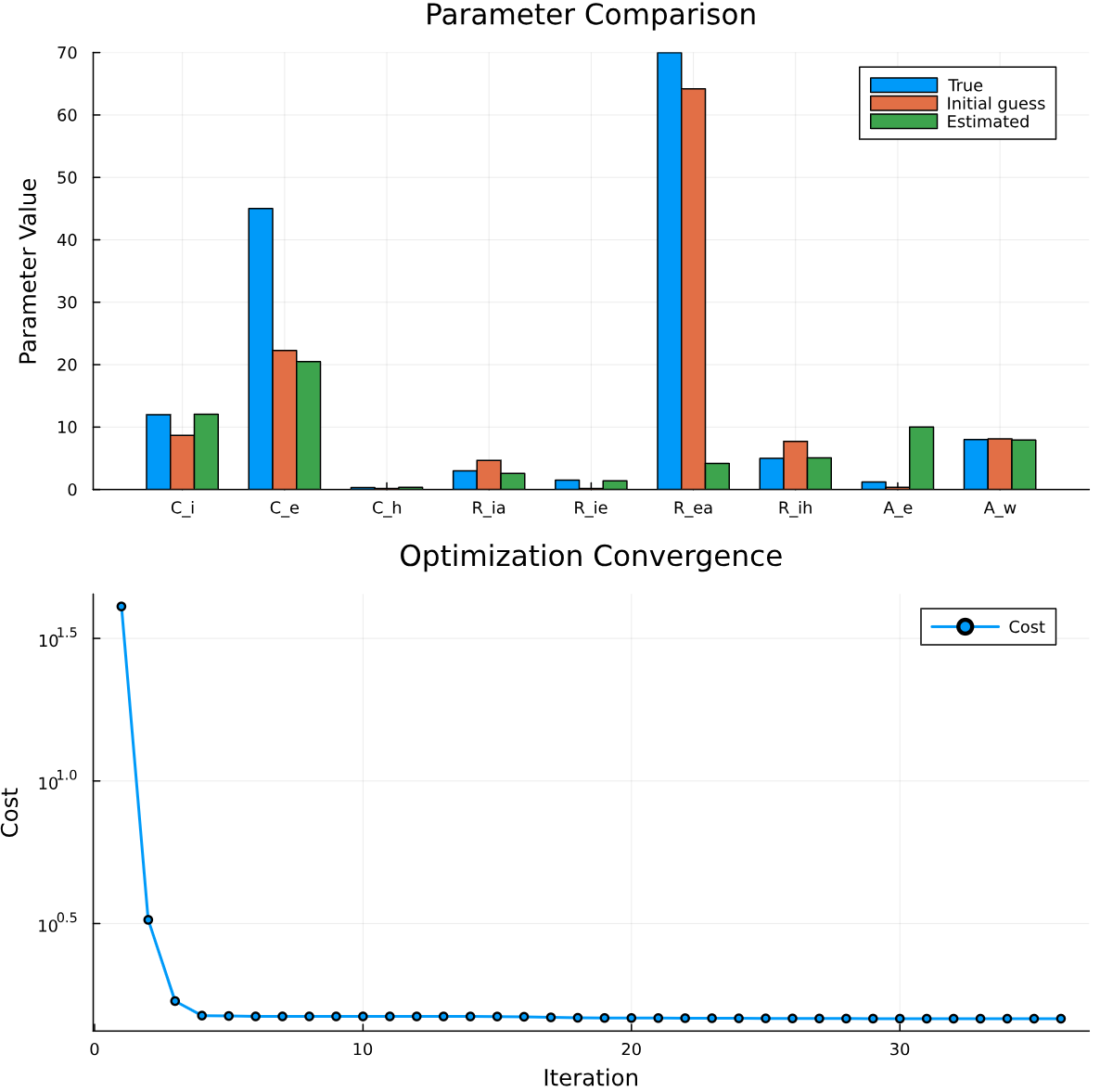
# plot parameter comparison
param_names = ["C_i", "C_e", "C_h", "R_ia", "R_ie", "R_ea", "R_ih", "A_e", "A_w"]
p1 = groupedbar(param_names, [p_true result.initial_guess result.parameters],
label=["True" "Initial guess" "Estimated"],
title="Parameter Comparison",
ylabel="Parameter Value",
legend=:topright, bar_width=0.7)
# plot cost convergence
p2 = plot(
result.cost_history,
xlabel="Iteration",
ylabel="Cost",
title="Optimization Convergence",
label="Cost",
linewidth=2,
yscale=:log10,
legend=:topright,
marker=:circle,
markersize=3
)
# combine plots
plot(p1, p2, layout=(2, 1), size=(1200, 800))
display(current())
I am not really sure why there is a sudden jump in the cost function trace and then afterwards it’s just flat.