Particle Filtering methods

Hi everyone! I’m new to data assimilation and working with particle filters. I have a model where the β function is sinusoidal and linearly advects over time. It’s a 2D field on an 80×80 grid with double bumps.

I’m trying to use BootstrapFilter() for this setup, but I haven’t been able to get it working. I did manage to run the example provided in particleFilter.jl, but not beyond that.

Has anyone used BootstrapFilter() for 2D fields or something similar? Any tips or examples would be really helpful!

The below is the code provided as an example but seemingly its not for 2D.

using Distributions # For probability distributions
using Random
using DelimitedFiles
using ParticleFilters
using VegaLite

# === System Parameters ===
# timestep
const dt = 0.2
# system nonlinearity, higher the value, more non-linear the state is 
const mu = 0.8
# standard deviation of the observation noise
const sigma = 0.6
# random number generator for reproducibility, Pseudorandom Number Generation:
# The Mersenne Twister is a pseudorandom number generator (PRNG), meaning it produces sequences of numbers that appear random but are actually generated by a deterministic algorithm
rng = MersenneTwister(1)

#  x = [x1, x2]
# === System Dynamics Function used to generate true data with some error to show real- word error (can be replaced with forward model)===
function f(x, u, rng)
    xdot = [x[2], mu * (1 - x[1]^2) * x[2] - x[1] + u + 0.01 * randn(rng)]
    return x + dt * xdot
end

#  observe only the first component x1 with gaussian noise. 
# too high sigma will make the observation too noisy and hard to assimilate (particles spread out too much)
# === Observation Function which are the observation + some random value ===
function h(x, rng)
    return x[1] + sigma * randn(rng)
end

# === Generate Synthetic Data ===
x = [3.0, 0.0] #initial state
k = 100 # number of time steps
xs = Array{typeof(x)}(undef, k) #stored true state trajectory

# exterbal control input
# in glacial model when the state is ice velocity, the control input is the subglacial water pressure or surface melt rate or external factors that affect the ice velocity
us = zeros(k) 
ys = zeros(k) #noisy observations
for t in 1:k
    global x
    x = f(x, us[t], rng)
    ys[t] = h(x, rng)
    xs[t] = x
end

# true state trajectory
writedlm("x.txt", xs)
# observations
writedlm("y.txt", ys)

writedlm("u.txt", us)
println("✅ Data files written: x.txt, y.txt, u.txt")

# this gives weight to particles based on their match with observations
g(x1, u, x2, y) = pdf(Normal(sigma), y - x2[1])
ys = vec(readdlm("y.txt"))
us = vec(readdlm("u.txt"))
xmat = readdlm("x.txt")

n = 10_000
fil = BootstrapFilter(f, g, n)

# Unweighted particle belief consisting of equally important particles of type (___)
# uniform prior on x1 belongin to [-5, 5] (NOT GAUSSIAN DISTRIBUTION) and x2 = 0
# initial particle belief on state
b0 = ParticleCollection([[10.0 * (rand() - 0.2), 0.0] for _ in 1:n])

# println("✅ Initial particle cloud saved to initial_particles.svg")

#  bs is the particle belief at each time step
# run the particle filter with the initial belief b0, control inputs us, and observations ys
# bs is a vector of ParticleCollection objects representing the particle beliefs at each time step
# each ParticleCollection contains particles representing the state of the system at that time step
bs = runfilter(fil, b0, us, ys)

# === Prepare Plotting Data ===
plot_data = [(; t, x1=x[1], x2=x[2], y, b_mean=mean(b)[1]) for (t, (x, y, b)) in enumerate(zip(eachslice(xmat; dims=1), ys, bs))]
println(plot_data)
# === Create Plot ===
plt = @vlplot(data=plot_data, width=700) +
      @vlplot(:line, x=:t, y=:x1, color={datum="True State"}) +
      @vlplot(:point, x=:t, y=:y, color={datum="Observation"}) +
      @vlplot(:line, x=:t, y=:b_mean, color={datum="Mean Belief"})


# === Getting root mean squared error ===
# ...existing code...

# === Getting root mean squared error ===
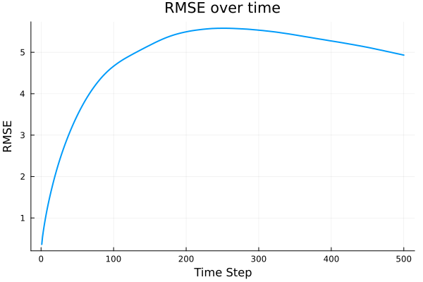
rmse = [sqrt(mean((b_mean - x1)^2)) for (; x1, b_mean) in plot_data]

rmse_data = [(; t, rmse=rmse[t]) for t in 1:length(rmse)]

rmse_plot = @vlplot(data=rmse_data, width=700) +
            @vlplot(:line, x=:t, y=:rmse, color={datum="RMSE"})

VegaLite.save("rmse.svg", rmse_plot)
println("✅ RMSE plot saved to rmse.svg")


VegaLite.save("myplot.svg", plt)
println("✅ Plot saved to myplot.pdf")

This example is running perfectly fine, but I’m not sure how to integrate my own 2D model with it. Below is my 2D model. To keep things simple, I’m using the analytical solution for linear advection to define the true model:

function generate_beta_field(grid::Grid, ω::Float64, t::Float64, v::Float64)
    x_shifted = grid.xxh .- v * t
    β = 1000 .+ 1000 .* sin.(ω .* x_shifted) .* sin.(ω .* grid.yyh)
    return β
end

# ------------------------------------------------------
# Simulate true beta field over time
# ------------------------------------------------------
function simulate_beta_motion(grid::Grid, ω::Float64, v::Float64; 
                              total_time::Float64=3600.0, dt::Float64=60.0)
    nt = Int(total_time / dt) + 1 # Include time 0 and total_time
    β_storage = Vector{Matrix{Float64}}()
    for i in 0:nt-1 # Loop through time steps 0 to nt-1
        t = i * dt
        β_t = generate_beta_field(grid, ω, t, v)
        push!(β_storage, β_t)
    end
    return β_storage
end

Also, I wanted to ask: is there another way I can perform particle filtering on this kind of model?

I came across the ParticleDA.jl package, which seems more general and supports things like multithreading and parallelization. But I’m not sure whether it’s possible (or advisable) to adapt it for my 2D analytical advection model. Has anyone tried using ParticleDA.jl with custom-defined models like this?

I’d love to hear if it’s flexible enough for such use cases, or if I should stick with writing a custom BootstrapFilter() pipeline from scratch.

Thanks in advance!

FWIW there’s also @baggepinnen 's Home · LowLevelParticleFilters Documentation

1 Like

Hi all,

I’m trying to apply a particle filtering algorithm to estimate the evolution of a spatial field, specifically:

β(x, y)=1000+1000⋅sin⁡(ωx)⋅sin⁡(ωy)

This β field is defined over a 2D grid (x, y) and has sinusoidal “bumps” in the z-direction. Conceptually, it is a scalar field distributed across a 2D spatial domain.

I’ve gone through the documentation of LowLevelParticleFilters.jl, which describes the algorithm in the standard state-space model form.

What I am struggling with is:
How to express my β field in a form that is compatible with the required state-space model.
Specifically, how to define the dynamics and measurement functions for a field defined on a grid (e.g., 80×80) instead of a low-dimensional vector.

I understand that in practice one can flatten the field to a long vector of length nx⋅ny, but conceptually it is unclear to me how this fits into the linear state-space formalism in the examples, since my field is not a moving “point” but rather a distributed quantity over space.

Has anyone applied LowLevelParticleFilters.jl (or particle filtering more generally) to track or estimate a spatial field like this?
Any guidance or examples on how to structure the state and dynamics in this context would be greatly appreciated.

Thanks in advance!

The equation you have posted for your scalar field \beta is not a dynamical equation, so there is no

Have you left something out? Is this supposed to be a PDE problem?

You need an equation that describes the dynamics of this field, i.e., how does the field change over time? Once you have established a partial-differential equation for this dynamics, you can discretize this in order to obtain a statespace representation of the dynamics that fits neatly into a filtering framework.

Here’s a simple example assuming that the dynamics is governed by advection one cell to the right

using LowLevelParticleFilters
using LinearAlgebra
using Statistics

# Grid and state
Nx, Ny = 30, 30
N = Nx * Ny

# Initial state
function initial_field()
    x = LinRange(0, 2π, Nx)
    y = LinRange(0, 2π, Ny)
    [sin(xi) * sin(2yi) for xi in x, yi in y] |> vec
end

# Dynamics: advection by 1 cell to the right
function dynamics(x, u, p, t)
    fmat = reshape(x, Nx, Ny)
    vec(circshift(fmat, (0, 1)))
end

# Observation: 100 random point samples
sensor_indices = rand(1:N, 100)
function measurement(x, u, p, t)
    x[sensor_indices]
end

# Covariances
R1 = 0.01^2 * I(N)  # small process noise
R2 = 0.1^2 * I(length(sensor_indices))  # observation noise

# Initialize EKF
x0 = initial_field()
P0 = I(N) * 0.1
d0 = LowLevelParticleFilters.SimpleMvNormal(x0, P0)

ekf = ExtendedKalmanFilter(
    dynamics, measurement, R1, R2, d0; nu=0
)

# Simulate true dynamics
T = 50
true_states = Vector{Vector{Float64}}(undef, T)
observations = Vector{Vector{Float64}}(undef, T)

x = x0
for t in 1:T
    global x
    x = dynamics(x, nothing, nothing, t) + 0.01 * randn(N)  # system evolution
    y = measurement(x, nothing, nothing, t) + 0.1 * randn(length(sensor_indices))  # observation
    true_states[t] = x
    observations[t] = y
end

# Run EKF
estimates = Vector{Vector{Float64}}(undef, T)
for t in 1:T
    update!(ekf, nothing, observations[t])
    estimates[t] = ekf.x
end

## A GIF animation of the evolution
using Plots
anim = @animate for t in 1:T
    plot(
        heatmap(reshape(true_states[t], Nx, Ny), title = "True State at t=$t"),
        heatmap(reshape(estimates[t], Nx, Ny), title = "EKF Estimate at t=$t"),
        size = (800, 400)
    )
end
gif(anim, "ekf_advection.gif", fps = 5)

ekf_advection

Please note, this uses an EKF instead of a particle filter, and a much coarser discretization to speed things up. To make this fast, provide a custom jacobian that exploits the sparsity properties of the problem:

julia> using SparseArrays

julia> sparse(ForwardDiff.jacobian(x->dynamics(x, nothing, nothing, 0.0), x0))
900×900 SparseMatrixCSC{Float64, Int64} with 900 stored entries:
⎡⠀⠀⠀⠀⠀⠀⠀⠀⠀⠀⠀⠀⠀⠀⠀⠀⠀⠀⠀⠀⠀⠀⠀⠀⠀⠀⠀⠀⠀⠀⠀⠀⠀⠀⠀⠀⠀⠀⠀⠀⠀⠀⠀⠀⠀⠀⠀⠀⠀⠀⠀⠀⠀⠀⠀⠀⠀⠀⠀⠀⠀⠀⠀⠀⠀⠀⠀⠀⠀⠀⠀⠀⠀⠀⠀⠀⠀⠀⠀⠀⠀⠳⣄⠀⎤
⎢⢤⡀⠀⠀⠀⠀⠀⠀⠀⠀⠀⠀⠀⠀⠀⠀⠀⠀⠀⠀⠀⠀⠀⠀⠀⠀⠀⠀⠀⠀⠀⠀⠀⠀⠀⠀⠀⠀⠀⠀⠀⠀⠀⠀⠀⠀⠀⠀⠀⠀⠀⠀⠀⠀⠀⠀⠀⠀⠀⠀⠀⠀⠀⠀⠀⠀⠀⠀⠀⠀⠀⠀⠀⠀⠀⠀⠀⠀⠀⠀⠀⠀⠈⠓⎥
⎢⠀⠙⢦⡀⠀⠀⠀⠀⠀⠀⠀⠀⠀⠀⠀⠀⠀⠀⠀⠀⠀⠀⠀⠀⠀⠀⠀⠀⠀⠀⠀⠀⠀⠀⠀⠀⠀⠀⠀⠀⠀⠀⠀⠀⠀⠀⠀⠀⠀⠀⠀⠀⠀⠀⠀⠀⠀⠀⠀⠀⠀⠀⠀⠀⠀⠀⠀⠀⠀⠀⠀⠀⠀⠀⠀⠀⠀⠀⠀⠀⠀⠀⠀⠀⎥
⎢⠀⠀⠀⠙⢦⡀⠀⠀⠀⠀⠀⠀⠀⠀⠀⠀⠀⠀⠀⠀⠀⠀⠀⠀⠀⠀⠀⠀⠀⠀⠀⠀⠀⠀⠀⠀⠀⠀⠀⠀⠀⠀⠀⠀⠀⠀⠀⠀⠀⠀⠀⠀⠀⠀⠀⠀⠀⠀⠀⠀⠀⠀⠀⠀⠀⠀⠀⠀⠀⠀⠀⠀⠀⠀⠀⠀⠀⠀⠀⠀⠀⠀⠀⠀⎥
⎢⠀⠀⠀⠀⠀⠙⢦⡀⠀⠀⠀⠀⠀⠀⠀⠀⠀⠀⠀⠀⠀⠀⠀⠀⠀⠀⠀⠀⠀⠀⠀⠀⠀⠀⠀⠀⠀⠀⠀⠀⠀⠀⠀⠀⠀⠀⠀⠀⠀⠀⠀⠀⠀⠀⠀⠀⠀⠀⠀⠀⠀⠀⠀⠀⠀⠀⠀⠀⠀⠀⠀⠀⠀⠀⠀⠀⠀⠀⠀⠀⠀⠀⠀⠀⎥
⎢⠀⠀⠀⠀⠀⠀⠀⠙⢦⡀⠀⠀⠀⠀⠀⠀⠀⠀⠀⠀⠀⠀⠀⠀⠀⠀⠀⠀⠀⠀⠀⠀⠀⠀⠀⠀⠀⠀⠀⠀⠀⠀⠀⠀⠀⠀⠀⠀⠀⠀⠀⠀⠀⠀⠀⠀⠀⠀⠀⠀⠀⠀⠀⠀⠀⠀⠀⠀⠀⠀⠀⠀⠀⠀⠀⠀⠀⠀⠀⠀⠀⠀⠀⠀⎥
⎢⠀⠀⠀⠀⠀⠀⠀⠀⠀⠙⢦⡀⠀⠀⠀⠀⠀⠀⠀⠀⠀⠀⠀⠀⠀⠀⠀⠀⠀⠀⠀⠀⠀⠀⠀⠀⠀⠀⠀⠀⠀⠀⠀⠀⠀⠀⠀⠀⠀⠀⠀⠀⠀⠀⠀⠀⠀⠀⠀⠀⠀⠀⠀⠀⠀⠀⠀⠀⠀⠀⠀⠀⠀⠀⠀⠀⠀⠀⠀⠀⠀⠀⠀⠀⎥
⎢⠀⠀⠀⠀⠀⠀⠀⠀⠀⠀⠀⠙⢦⡀⠀⠀⠀⠀⠀⠀⠀⠀⠀⠀⠀⠀⠀⠀⠀⠀⠀⠀⠀⠀⠀⠀⠀⠀⠀⠀⠀⠀⠀⠀⠀⠀⠀⠀⠀⠀⠀⠀⠀⠀⠀⠀⠀⠀⠀⠀⠀⠀⠀⠀⠀⠀⠀⠀⠀⠀⠀⠀⠀⠀⠀⠀⠀⠀⠀⠀⠀⠀⠀⠀⎥
⎢⠀⠀⠀⠀⠀⠀⠀⠀⠀⠀⠀⠀⠀⠙⢦⡀⠀⠀⠀⠀⠀⠀⠀⠀⠀⠀⠀⠀⠀⠀⠀⠀⠀⠀⠀⠀⠀⠀⠀⠀⠀⠀⠀⠀⠀⠀⠀⠀⠀⠀⠀⠀⠀⠀⠀⠀⠀⠀⠀⠀⠀⠀⠀⠀⠀⠀⠀⠀⠀⠀⠀⠀⠀⠀⠀⠀⠀⠀⠀⠀⠀⠀⠀⠀⎥
⎢⠀⠀⠀⠀⠀⠀⠀⠀⠀⠀⠀⠀⠀⠀⠀⠙⢦⡀⠀⠀⠀⠀⠀⠀⠀⠀⠀⠀⠀⠀⠀⠀⠀⠀⠀⠀⠀⠀⠀⠀⠀⠀⠀⠀⠀⠀⠀⠀⠀⠀⠀⠀⠀⠀⠀⠀⠀⠀⠀⠀⠀⠀⠀⠀⠀⠀⠀⠀⠀⠀⠀⠀⠀⠀⠀⠀⠀⠀⠀⠀⠀⠀⠀⠀⎥
⎢⠀⠀⠀⠀⠀⠀⠀⠀⠀⠀⠀⠀⠀⠀⠀⠀⠀⠙⢦⡀⠀⠀⠀⠀⠀⠀⠀⠀⠀⠀⠀⠀⠀⠀⠀⠀⠀⠀⠀⠀⠀⠀⠀⠀⠀⠀⠀⠀⠀⠀⠀⠀⠀⠀⠀⠀⠀⠀⠀⠀⠀⠀⠀⠀⠀⠀⠀⠀⠀⠀⠀⠀⠀⠀⠀⠀⠀⠀⠀⠀⠀⠀⠀⠀⎥
⎢⠀⠀⠀⠀⠀⠀⠀⠀⠀⠀⠀⠀⠀⠀⠀⠀⠀⠀⠀⠙⢦⡀⠀⠀⠀⠀⠀⠀⠀⠀⠀⠀⠀⠀⠀⠀⠀⠀⠀⠀⠀⠀⠀⠀⠀⠀⠀⠀⠀⠀⠀⠀⠀⠀⠀⠀⠀⠀⠀⠀⠀⠀⠀⠀⠀⠀⠀⠀⠀⠀⠀⠀⠀⠀⠀⠀⠀⠀⠀⠀⠀⠀⠀⠀⎥
⎢⠀⠀⠀⠀⠀⠀⠀⠀⠀⠀⠀⠀⠀⠀⠀⠀⠀⠀⠀⠀⠀⠙⢦⡀⠀⠀⠀⠀⠀⠀⠀⠀⠀⠀⠀⠀⠀⠀⠀⠀⠀⠀⠀⠀⠀⠀⠀⠀⠀⠀⠀⠀⠀⠀⠀⠀⠀⠀⠀⠀⠀⠀⠀⠀⠀⠀⠀⠀⠀⠀⠀⠀⠀⠀⠀⠀⠀⠀⠀⠀⠀⠀⠀⠀⎥
⎢⠀⠀⠀⠀⠀⠀⠀⠀⠀⠀⠀⠀⠀⠀⠀⠀⠀⠀⠀⠀⠀⠀⠀⠙⢦⡀⠀⠀⠀⠀⠀⠀⠀⠀⠀⠀⠀⠀⠀⠀⠀⠀⠀⠀⠀⠀⠀⠀⠀⠀⠀⠀⠀⠀⠀⠀⠀⠀⠀⠀⠀⠀⠀⠀⠀⠀⠀⠀⠀⠀⠀⠀⠀⠀⠀⠀⠀⠀⠀⠀⠀⠀⠀⠀⎥
⎢⠀⠀⠀⠀⠀⠀⠀⠀⠀⠀⠀⠀⠀⠀⠀⠀⠀⠀⠀⠀⠀⠀⠀⠀⠀⠙⢦⡀⠀⠀⠀⠀⠀⠀⠀⠀⠀⠀⠀⠀⠀⠀⠀⠀⠀⠀⠀⠀⠀⠀⠀⠀⠀⠀⠀⠀⠀⠀⠀⠀⠀⠀⠀⠀⠀⠀⠀⠀⠀⠀⠀⠀⠀⠀⠀⠀⠀⠀⠀⠀⠀⠀⠀⠀⎥
⎢⠀⠀⠀⠀⠀⠀⠀⠀⠀⠀⠀⠀⠀⠀⠀⠀⠀⠀⠀⠀⠀⠀⠀⠀⠀⠀⠀⠙⢦⡀⠀⠀⠀⠀⠀⠀⠀⠀⠀⠀⠀⠀⠀⠀⠀⠀⠀⠀⠀⠀⠀⠀⠀⠀⠀⠀⠀⠀⠀⠀⠀⠀⠀⠀⠀⠀⠀⠀⠀⠀⠀⠀⠀⠀⠀⠀⠀⠀⠀⠀⠀⠀⠀⠀⎥
⎢⠀⠀⠀⠀⠀⠀⠀⠀⠀⠀⠀⠀⠀⠀⠀⠀⠀⠀⠀⠀⠀⠀⠀⠀⠀⠀⠀⠀⠀⠙⢦⡀⠀⠀⠀⠀⠀⠀⠀⠀⠀⠀⠀⠀⠀⠀⠀⠀⠀⠀⠀⠀⠀⠀⠀⠀⠀⠀⠀⠀⠀⠀⠀⠀⠀⠀⠀⠀⠀⠀⠀⠀⠀⠀⠀⠀⠀⠀⠀⠀⠀⠀⠀⠀⎥
⎢⠀⠀⠀⠀⠀⠀⠀⠀⠀⠀⠀⠀⠀⠀⠀⠀⠀⠀⠀⠀⠀⠀⠀⠀⠀⠀⠀⠀⠀⠀⠀⠙⢦⡀⠀⠀⠀⠀⠀⠀⠀⠀⠀⠀⠀⠀⠀⠀⠀⠀⠀⠀⠀⠀⠀⠀⠀⠀⠀⠀⠀⠀⠀⠀⠀⠀⠀⠀⠀⠀⠀⠀⠀⠀⠀⠀⠀⠀⠀⠀⠀⠀⠀⠀⎥
⎢⠀⠀⠀⠀⠀⠀⠀⠀⠀⠀⠀⠀⠀⠀⠀⠀⠀⠀⠀⠀⠀⠀⠀⠀⠀⠀⠀⠀⠀⠀⠀⠀⠀⠙⢦⡀⠀⠀⠀⠀⠀⠀⠀⠀⠀⠀⠀⠀⠀⠀⠀⠀⠀⠀⠀⠀⠀⠀⠀⠀⠀⠀⠀⠀⠀⠀⠀⠀⠀⠀⠀⠀⠀⠀⠀⠀⠀⠀⠀⠀⠀⠀⠀⠀⎥
⎢⠀⠀⠀⠀⠀⠀⠀⠀⠀⠀⠀⠀⠀⠀⠀⠀⠀⠀⠀⠀⠀⠀⠀⠀⠀⠀⠀⠀⠀⠀⠀⠀⠀⠀⠀⠙⢦⡀⠀⠀⠀⠀⠀⠀⠀⠀⠀⠀⠀⠀⠀⠀⠀⠀⠀⠀⠀⠀⠀⠀⠀⠀⠀⠀⠀⠀⠀⠀⠀⠀⠀⠀⠀⠀⠀⠀⠀⠀⠀⠀⠀⠀⠀⠀⎥
⎢⠀⠀⠀⠀⠀⠀⠀⠀⠀⠀⠀⠀⠀⠀⠀⠀⠀⠀⠀⠀⠀⠀⠀⠀⠀⠀⠀⠀⠀⠀⠀⠀⠀⠀⠀⠀⠀⠙⢦⡀⠀⠀⠀⠀⠀⠀⠀⠀⠀⠀⠀⠀⠀⠀⠀⠀⠀⠀⠀⠀⠀⠀⠀⠀⠀⠀⠀⠀⠀⠀⠀⠀⠀⠀⠀⠀⠀⠀⠀⠀⠀⠀⠀⠀⎥
⎢⠀⠀⠀⠀⠀⠀⠀⠀⠀⠀⠀⠀⠀⠀⠀⠀⠀⠀⠀⠀⠀⠀⠀⠀⠀⠀⠀⠀⠀⠀⠀⠀⠀⠀⠀⠀⠀⠀⠀⠙⢦⡀⠀⠀⠀⠀⠀⠀⠀⠀⠀⠀⠀⠀⠀⠀⠀⠀⠀⠀⠀⠀⠀⠀⠀⠀⠀⠀⠀⠀⠀⠀⠀⠀⠀⠀⠀⠀⠀⠀⠀⠀⠀⠀⎥
⎢⠀⠀⠀⠀⠀⠀⠀⠀⠀⠀⠀⠀⠀⠀⠀⠀⠀⠀⠀⠀⠀⠀⠀⠀⠀⠀⠀⠀⠀⠀⠀⠀⠀⠀⠀⠀⠀⠀⠀⠀⠀⠙⢦⡀⠀⠀⠀⠀⠀⠀⠀⠀⠀⠀⠀⠀⠀⠀⠀⠀⠀⠀⠀⠀⠀⠀⠀⠀⠀⠀⠀⠀⠀⠀⠀⠀⠀⠀⠀⠀⠀⠀⠀⠀⎥
⎢⠀⠀⠀⠀⠀⠀⠀⠀⠀⠀⠀⠀⠀⠀⠀⠀⠀⠀⠀⠀⠀⠀⠀⠀⠀⠀⠀⠀⠀⠀⠀⠀⠀⠀⠀⠀⠀⠀⠀⠀⠀⠀⠀⠙⢦⡀⠀⠀⠀⠀⠀⠀⠀⠀⠀⠀⠀⠀⠀⠀⠀⠀⠀⠀⠀⠀⠀⠀⠀⠀⠀⠀⠀⠀⠀⠀⠀⠀⠀⠀⠀⠀⠀⠀⎥
⎢⠀⠀⠀⠀⠀⠀⠀⠀⠀⠀⠀⠀⠀⠀⠀⠀⠀⠀⠀⠀⠀⠀⠀⠀⠀⠀⠀⠀⠀⠀⠀⠀⠀⠀⠀⠀⠀⠀⠀⠀⠀⠀⠀⠀⠀⠙⢦⡀⠀⠀⠀⠀⠀⠀⠀⠀⠀⠀⠀⠀⠀⠀⠀⠀⠀⠀⠀⠀⠀⠀⠀⠀⠀⠀⠀⠀⠀⠀⠀⠀⠀⠀⠀⠀⎥
⎢⠀⠀⠀⠀⠀⠀⠀⠀⠀⠀⠀⠀⠀⠀⠀⠀⠀⠀⠀⠀⠀⠀⠀⠀⠀⠀⠀⠀⠀⠀⠀⠀⠀⠀⠀⠀⠀⠀⠀⠀⠀⠀⠀⠀⠀⠀⠀⠙⢦⡀⠀⠀⠀⠀⠀⠀⠀⠀⠀⠀⠀⠀⠀⠀⠀⠀⠀⠀⠀⠀⠀⠀⠀⠀⠀⠀⠀⠀⠀⠀⠀⠀⠀⠀⎥
⎢⠀⠀⠀⠀⠀⠀⠀⠀⠀⠀⠀⠀⠀⠀⠀⠀⠀⠀⠀⠀⠀⠀⠀⠀⠀⠀⠀⠀⠀⠀⠀⠀⠀⠀⠀⠀⠀⠀⠀⠀⠀⠀⠀⠀⠀⠀⠀⠀⠀⠙⢦⡀⠀⠀⠀⠀⠀⠀⠀⠀⠀⠀⠀⠀⠀⠀⠀⠀⠀⠀⠀⠀⠀⠀⠀⠀⠀⠀⠀⠀⠀⠀⠀⠀⎥
⎢⠀⠀⠀⠀⠀⠀⠀⠀⠀⠀⠀⠀⠀⠀⠀⠀⠀⠀⠀⠀⠀⠀⠀⠀⠀⠀⠀⠀⠀⠀⠀⠀⠀⠀⠀⠀⠀⠀⠀⠀⠀⠀⠀⠀⠀⠀⠀⠀⠀⠀⠀⠙⢦⡀⠀⠀⠀⠀⠀⠀⠀⠀⠀⠀⠀⠀⠀⠀⠀⠀⠀⠀⠀⠀⠀⠀⠀⠀⠀⠀⠀⠀⠀⠀⎥
⎢⠀⠀⠀⠀⠀⠀⠀⠀⠀⠀⠀⠀⠀⠀⠀⠀⠀⠀⠀⠀⠀⠀⠀⠀⠀⠀⠀⠀⠀⠀⠀⠀⠀⠀⠀⠀⠀⠀⠀⠀⠀⠀⠀⠀⠀⠀⠀⠀⠀⠀⠀⠀⠀⠙⢦⡀⠀⠀⠀⠀⠀⠀⠀⠀⠀⠀⠀⠀⠀⠀⠀⠀⠀⠀⠀⠀⠀⠀⠀⠀⠀⠀⠀⠀⎥
⎢⠀⠀⠀⠀⠀⠀⠀⠀⠀⠀⠀⠀⠀⠀⠀⠀⠀⠀⠀⠀⠀⠀⠀⠀⠀⠀⠀⠀⠀⠀⠀⠀⠀⠀⠀⠀⠀⠀⠀⠀⠀⠀⠀⠀⠀⠀⠀⠀⠀⠀⠀⠀⠀⠀⠀⠙⢦⡀⠀⠀⠀⠀⠀⠀⠀⠀⠀⠀⠀⠀⠀⠀⠀⠀⠀⠀⠀⠀⠀⠀⠀⠀⠀⠀⎥
⎢⠀⠀⠀⠀⠀⠀⠀⠀⠀⠀⠀⠀⠀⠀⠀⠀⠀⠀⠀⠀⠀⠀⠀⠀⠀⠀⠀⠀⠀⠀⠀⠀⠀⠀⠀⠀⠀⠀⠀⠀⠀⠀⠀⠀⠀⠀⠀⠀⠀⠀⠀⠀⠀⠀⠀⠀⠀⠙⢦⡀⠀⠀⠀⠀⠀⠀⠀⠀⠀⠀⠀⠀⠀⠀⠀⠀⠀⠀⠀⠀⠀⠀⠀⠀⎥
⎢⠀⠀⠀⠀⠀⠀⠀⠀⠀⠀⠀⠀⠀⠀⠀⠀⠀⠀⠀⠀⠀⠀⠀⠀⠀⠀⠀⠀⠀⠀⠀⠀⠀⠀⠀⠀⠀⠀⠀⠀⠀⠀⠀⠀⠀⠀⠀⠀⠀⠀⠀⠀⠀⠀⠀⠀⠀⠀⠀⠙⢦⡀⠀⠀⠀⠀⠀⠀⠀⠀⠀⠀⠀⠀⠀⠀⠀⠀⠀⠀⠀⠀⠀⠀⎥
⎢⠀⠀⠀⠀⠀⠀⠀⠀⠀⠀⠀⠀⠀⠀⠀⠀⠀⠀⠀⠀⠀⠀⠀⠀⠀⠀⠀⠀⠀⠀⠀⠀⠀⠀⠀⠀⠀⠀⠀⠀⠀⠀⠀⠀⠀⠀⠀⠀⠀⠀⠀⠀⠀⠀⠀⠀⠀⠀⠀⠀⠀⠙⢦⡀⠀⠀⠀⠀⠀⠀⠀⠀⠀⠀⠀⠀⠀⠀⠀⠀⠀⠀⠀⠀⎥
⎢⠀⠀⠀⠀⠀⠀⠀⠀⠀⠀⠀⠀⠀⠀⠀⠀⠀⠀⠀⠀⠀⠀⠀⠀⠀⠀⠀⠀⠀⠀⠀⠀⠀⠀⠀⠀⠀⠀⠀⠀⠀⠀⠀⠀⠀⠀⠀⠀⠀⠀⠀⠀⠀⠀⠀⠀⠀⠀⠀⠀⠀⠀⠀⠙⢦⡀⠀⠀⠀⠀⠀⠀⠀⠀⠀⠀⠀⠀⠀⠀⠀⠀⠀⠀⎥
⎢⠀⠀⠀⠀⠀⠀⠀⠀⠀⠀⠀⠀⠀⠀⠀⠀⠀⠀⠀⠀⠀⠀⠀⠀⠀⠀⠀⠀⠀⠀⠀⠀⠀⠀⠀⠀⠀⠀⠀⠀⠀⠀⠀⠀⠀⠀⠀⠀⠀⠀⠀⠀⠀⠀⠀⠀⠀⠀⠀⠀⠀⠀⠀⠀⠀⠙⢦⡀⠀⠀⠀⠀⠀⠀⠀⠀⠀⠀⠀⠀⠀⠀⠀⠀⎥
⎢⠀⠀⠀⠀⠀⠀⠀⠀⠀⠀⠀⠀⠀⠀⠀⠀⠀⠀⠀⠀⠀⠀⠀⠀⠀⠀⠀⠀⠀⠀⠀⠀⠀⠀⠀⠀⠀⠀⠀⠀⠀⠀⠀⠀⠀⠀⠀⠀⠀⠀⠀⠀⠀⠀⠀⠀⠀⠀⠀⠀⠀⠀⠀⠀⠀⠀⠀⠙⢦⡀⠀⠀⠀⠀⠀⠀⠀⠀⠀⠀⠀⠀⠀⠀⎥
⎢⠀⠀⠀⠀⠀⠀⠀⠀⠀⠀⠀⠀⠀⠀⠀⠀⠀⠀⠀⠀⠀⠀⠀⠀⠀⠀⠀⠀⠀⠀⠀⠀⠀⠀⠀⠀⠀⠀⠀⠀⠀⠀⠀⠀⠀⠀⠀⠀⠀⠀⠀⠀⠀⠀⠀⠀⠀⠀⠀⠀⠀⠀⠀⠀⠀⠀⠀⠀⠀⠙⢦⡀⠀⠀⠀⠀⠀⠀⠀⠀⠀⠀⠀⠀⎥
⎢⠀⠀⠀⠀⠀⠀⠀⠀⠀⠀⠀⠀⠀⠀⠀⠀⠀⠀⠀⠀⠀⠀⠀⠀⠀⠀⠀⠀⠀⠀⠀⠀⠀⠀⠀⠀⠀⠀⠀⠀⠀⠀⠀⠀⠀⠀⠀⠀⠀⠀⠀⠀⠀⠀⠀⠀⠀⠀⠀⠀⠀⠀⠀⠀⠀⠀⠀⠀⠀⠀⠀⠙⢦⡀⠀⠀⠀⠀⠀⠀⠀⠀⠀⠀⎥
⎢⠀⠀⠀⠀⠀⠀⠀⠀⠀⠀⠀⠀⠀⠀⠀⠀⠀⠀⠀⠀⠀⠀⠀⠀⠀⠀⠀⠀⠀⠀⠀⠀⠀⠀⠀⠀⠀⠀⠀⠀⠀⠀⠀⠀⠀⠀⠀⠀⠀⠀⠀⠀⠀⠀⠀⠀⠀⠀⠀⠀⠀⠀⠀⠀⠀⠀⠀⠀⠀⠀⠀⠀⠀⠙⢦⡀⠀⠀⠀⠀⠀⠀⠀⠀⎥
⎢⠀⠀⠀⠀⠀⠀⠀⠀⠀⠀⠀⠀⠀⠀⠀⠀⠀⠀⠀⠀⠀⠀⠀⠀⠀⠀⠀⠀⠀⠀⠀⠀⠀⠀⠀⠀⠀⠀⠀⠀⠀⠀⠀⠀⠀⠀⠀⠀⠀⠀⠀⠀⠀⠀⠀⠀⠀⠀⠀⠀⠀⠀⠀⠀⠀⠀⠀⠀⠀⠀⠀⠀⠀⠀⠀⠙⢦⡀⠀⠀⠀⠀⠀⠀⎥
⎢⠀⠀⠀⠀⠀⠀⠀⠀⠀⠀⠀⠀⠀⠀⠀⠀⠀⠀⠀⠀⠀⠀⠀⠀⠀⠀⠀⠀⠀⠀⠀⠀⠀⠀⠀⠀⠀⠀⠀⠀⠀⠀⠀⠀⠀⠀⠀⠀⠀⠀⠀⠀⠀⠀⠀⠀⠀⠀⠀⠀⠀⠀⠀⠀⠀⠀⠀⠀⠀⠀⠀⠀⠀⠀⠀⠀⠀⠙⢦⡀⠀⠀⠀⠀⎥
⎣⠀⠀⠀⠀⠀⠀⠀⠀⠀⠀⠀⠀⠀⠀⠀⠀⠀⠀⠀⠀⠀⠀⠀⠀⠀⠀⠀⠀⠀⠀⠀⠀⠀⠀⠀⠀⠀⠀⠀⠀⠀⠀⠀⠀⠀⠀⠀⠀⠀⠀⠀⠀⠀⠀⠀⠀⠀⠀⠀⠀⠀⠀⠀⠀⠀⠀⠀⠀⠀⠀⠀⠀⠀⠀⠀⠀⠀⠀⠀⠙⢦⠀⠀⠀⎦
4 Likes

For completeness, here’s an example that sets up the sparse jacobians. With this, I can push it to a 50x50 grid, but beyond that it becomes quite expensive. For large PDE problems, Ensemble Kalman filtering is commonly employed for this reason. There are still a lot of room for optimization of the performance here, for example, one may use in-place updates of the dynamics and measurement functions to prevent excessive memory allocations.

using LowLevelParticleFilters
using LinearAlgebra
using Random
using Statistics
using SparseConnectivityTracer, SparseMatrixColorings, ForwardDiff, DifferentiationInterface

# Grid and state
Nx, Ny = 50, 50
N = Nx * Ny

# Initial state
function initial_field()
    x = LinRange(0, 2π, Nx)
    y = LinRange(0, 2π, Ny)
    [sin(xi) * sin(2yi) for xi in x, yi in y] |> vec
end

# Dynamics: advection by 1 cell to the right
function dynamics(x, u, p, t)
    fmat = reshape(x, Nx, Ny)
    vec(circshift(fmat, (0, 1)))
end

# Observation: 100 random point samples
sensor_indices = rand(1:N, 100)
function measurement(x, u, p, t)
    x[sensor_indices]
end

# Covariances
R1 = 0.01^2 * I(N)  # small process noise
R2 = 0.1^2 * I(length(sensor_indices))  # observation noise

# Initialize EKF
x0 = initial_field()
P0 = I(N) * 0.1
d0 = LowLevelParticleFilters.SimpleMvNormal(x0, P0)

## Set up sparse jacobian using DifferentiationInterface for dynamics
f(x) = dynamics(x, nothing, nothing, 0)
backend = AutoSparse(AutoForwardDiff())
prep = prepare_jacobian(f, backend, zero(x0))
grad = similar(x0*x0')
Ajac(x,u,p,t) = jacobian!(f, grad, prep, backend, x)

## Set up sparse jacobian using DifferentiationInterface for measurement
h(x) = measurement(x, nothing, nothing, 0)
prep_meas = prepare_jacobian(h, backend, zero(x0))
grad_meas = similar(h(x0)*x0')
Cjac(x,u,p,t) = jacobian!(h, grad_meas, prep_meas, backend, x)

ekf = ExtendedKalmanFilter(
    dynamics, measurement, R1, R2, d0; nu=0, Ajac, Cjac,
)

# Simulate true dynamics
T = 50
true_states = Vector{Vector{Float64}}(undef, T)
observations = Vector{Vector{Float64}}(undef, T)

x = x0
for t in 1:T
    global x
    x = dynamics(x, nothing, nothing, t) + 0.01 * randn(N)  # system evolution
    y = measurement(x, nothing, nothing, t) + 0.1 * randn(length(sensor_indices))  # observation
    true_states[t] = x
    observations[t] = y
end

# Run EKF
estimates = Vector{Vector{Float64}}(undef, T)
for t in 1:T
    @show t
    update!(ekf, nothing, observations[t])
    estimates[t] = ekf.x
end

## A GIF animation of the evolution
using Plots
anim = @animate for t in 1:T
    plot(
        heatmap(reshape(true_states[t], Nx, Ny), title = "True State at t=$t"),
        heatmap(reshape(estimates[t], Nx, Ny), title = "EKF Estimate at t=$t"),
        size = (800, 400)
    )
end
gif(anim, "ekf_advection.gif", fps = 5)

ekf_advection

4 Likes

Thanks for sharing the full dynamics and EnKF code — that was really helpful! If I eventually move to non-linear advection PDE/dynamics for the same problem, can a similar approach still work? I’ve read that particle filters can perform better than EnKF in non-linear settings. Would you recommend trying PF here, or sticking with EnKF?
Also i tried plotting RMSE for the same, and it seems like its increasing with time. Shouldn’t it be decreasing over time as the filter will become more closer to the actual truth. Thanks again for your guidance!

The code I provided uses a standard EKF (Extended Kalman filter), I have no implementation of Ensemble Kalman filters at hand.

Yes, EKF and particle filters both handle nonlinear dynamics.

The state dimension is very large, particle filter may struggle with such a high state dimension. I have no experience applying them in this context so I can’t give you more than this general advice.

It is generally true that particle filters can handle more challenging nonlinearities than Ensemble Kalman filters, but as the state dimension gets large they suffer from the curse of dimensionality. What are your performace requirements here? An EKF (note, not EnKF) can perhaps work if performance requirements are modest.

1 Like

I tried running the Extended Kalman Filter code you provided and computed the RMSE over time. However, I am unable to understand the reason behind the vague RMSE trend I am observing:

Shouldn’t the RMSE generally decrease or stabilize over time as the filter assimilates more observations, rather than increasing as shown here? Any insights on what might be causing this behavior would be greatly appreciated.

It depends on how large the uncertainty is in the initial distribution compared to the stationary distribution. If you push that example much further in time, it might converge. You can compute the stationary covariance matrix by solving a Riccati equation with the A jacobian, see Influence of sample rate on performance · LowLevelParticleFilters Documentation for some details or “Asymptotic form” in Kalman filter - Wikipedia

using MatrixEquations
A = Ajac(...)
C = Cjac(...)
R_stationary, _ = ared(A, C', R2, R1)

or something like that.

You are essentially plotting the evolution of the equation

X^+ = A X A^T - (A XB)(R_2+B^T XB)^{-1}(B^T XA^T) + R_1

where B = C^T, and you might not have plotted enough evolution of it for it to converge.

1 Like