Wait a second…
In your MATLAB script you did:
options = odeset('Reltol',1e-6);
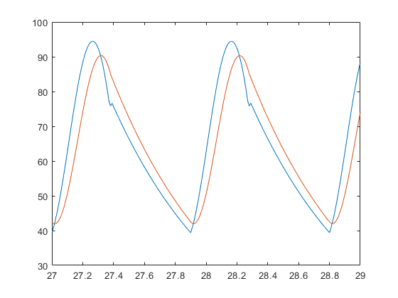
If you don’t change the default reltol then you get:
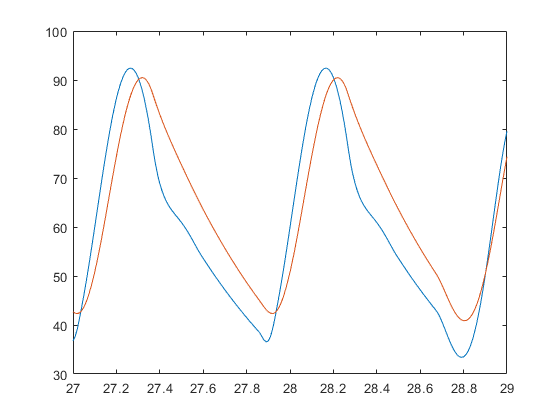
It’s only after you change to reltol=1e-6 that you get:
So it does require that you drop the reltol a little bit! And if you do that in Julia, it similarly works:
@time sol = solve(problem,DP5(),reltol=1e-6)
@time sola = solve(problem,Tsit5(),abstol=1e-12,reltol=1e-12)
length(sol) # 1368
plot(sol,tspan=(27.0,29.0))
plot!(sola,tspan=(27.0,29.0))
savefig("plot4.png")

which solves in 0.041426 seconds (1.50 M allocations: 23.584 MiB)
So why is your Julia code so slow? It’s because I_generic has a ton of non-constant globals in it, so it’s not type stable. So fix that and:
0.002944 seconds (8.27 k allocations: 870.594 KiB)
Ahh, that’s better.
Final code:
using OrdinaryDiffEq
function wk5(dP, P, params, t)

    #=

    The 5-Element WK with serial L
    set Ls = 0 for 4-Element WK parallel

    Formulation for DifferentialEquations.jl

    P:          solution vector (pressures p1 and p2)
    params: parameter array
                [ Rc, Rp, C, Lp, Ls ]


    I need to find a way to tranfer the function name as well
    for the time being we have to have the function in "I"

    =#

    # Split parameter array:
    Rc, Rp, C, Lp, Ls = params

    dP[1] = (
        -Rc / Lp * P[1]
        + (Rc / Lp - 1 / Rp / C) * P[2]
        + Rc * (1 + Ls / Lp) * didt(I, t)
        + I(t) / C
        )

    dP[2] = -1 / Rp / C * P[2] + I(t) / C
end

# Generic Input Waveform
# max volume flow in ml/s
const max_i = 425

# min volume flow in m^3/s
const min_i = 0.0
const T = 0.9

# Syst. Time in s
const systTime = 2 / 5 * T

# Dicrotic notch time
const dicrTime = 0.02


function I_generic(t)
  # implicit conditional using boolean multiplicator
  # sine waveform
  (
      (max_i - min_i) * sin(pi / systTime * (t % T))
      * (t % T < (systTime + dicrTime) )
      + min_i
  )
end

function didt(I, t)
    dt = 1e-3;
    didt = (I(t+dt) - I(t-dt)) / (2 * dt);
    return didt
end

# Initial condition and time span
P0 = [0.0, 0.0]
tspan = (0.0, 30.0)

# Set parameters for Windkessel Model
Rc = 0.033
Rp = 0.6
C = 1.25
# L for serial model!
Ls = 0.01
# L for parallel
Lp = 0.02
p5 = [Rc, Rp, C, Lp, Ls]

const I = I_generic
problem = ODEProblem(wk5, P0, tspan, p5)
@time solutionDP5 = solve(problem,DP5(), reltol=1e-6)
# 0.002944 seconds (8.27 k allocations: 870.594 KiB)
using Plots
plot(solutionDP5,tspan=(27.0,29.0))
savefig("plot1.png")