This is my first post in a Julia forum! I have really been enjoying studying Turing.jl , Gen, and Julia in general. Thank you to all developers!
I am trying to fit a simple “logit normal” model, that is a typical Binomial model where the probabilities vary between trials. This variation is modeled as a normal distribution on the logit scale. I’m including a reproducible example below. When I run this in Julia 1.2.0 i get a large number of numerical errors, followed by what appears to be a single sample from the posterior (not 2000, as I had hoped). Any help would be appreciated !
ns = fill(400, 50)

# Sigmoid function (numerically stable)
sigmoid(x::T) where {T<:Real} = x >= zero(x) ? inv(exp(-x) + one(x)) : exp(x) / (exp(x) + one(x))

# variation in probabilities
ps = sigmoid.(rand(Normal(-1,0.5), 50))

xs = rand.(Binomial.(ns, ps))


@model normal_logit(n, x) = begin
    n_obs = length(n)

    ## hyperparameters for varying effectgs
    ā ~ Normal(0, 0.5)
    σ_a ~ Truncated(Exponential(3), 0, Inf)

    # varying intercepts for each observation
    a = Vector{Real}(undef, n_obs)
    a ~ [Normal(ā, σ_a)]
    p = sigmoid.(a)

    for i in eachindex(n)
        x[i] ~ Binomial(n[i], p[i])
    end
end


normal_logit_samples = sample(normal_logit(xs, ps), NUTS(100, 0.65), 2000)
Regarding your question. The sigmoid function is unfortunately not numerically stable. Therefore, we provide the BinomialLogit distribution as a numerically stable alternative in Turing.
Btw. You can probably significantly improve the performance of sampling by using reverse mode AD and making the model type stable.
See this example:
@model gauss2(x, ::Type{TV}=Vector{Float64}) where {TV} = begin
            priors = TV(undef, 2)
            priors[1] ~ InverseGamma(2,3)         # s
            priors[2] ~ Normal(0, sqrt(priors[1])) # m
            for i in 1:length(x)
                x[i] ~ Normal(priors[2], sqrt(priors[1]))
            end
        end
In your case you would replace the Array{Real} by the TV syntax used above.
Apologies for the short responses, I’m writing on the phone.
Thank you everyone who answered! after including all your suggestions I still receive many thousands of numerical errors. when the sampler does “finish”, there seems to be only a single effective sample (at least, the errors are on the order of e-17) !
Here is one of my error messages:
┌ Warning: The current proposal will be rejected due to numerical error(s).
│   isfiniteθ = true
│   isfiniter = true
│   isfiniteℓπ = false
│   isfiniteℓκ = true
└ @ AdvancedHMC ~/.julia/packages/AdvancedHMC/PQWco/src/hamiltonian.jl:36
And here is a part of the result (incidentally, the estimates are not at all close to the values used in simulation)
I’m struggling to understand your model. But I think at the moment it is not correctly implemented.
I think it might be like this, but I’m not 100% sure what you aim to do.
# your model
# n: number of trials for each observation
# x: observed value
@model normal_logit(n, x) = begin

    n_obs = length(n)

    ## hyperparameters for varying effectgs
    ā ~ Normal(0, 0.5)
    σ_a ~ Truncated(Exponential(3), 0, Inf)

    # varying intercepts for each observation
    a ~ MvNormal(fill(ā, n_obs), σ_a)

    for i in eachindex(n)
        x[i] ~ BinomialLogit(n[i], a[i])
    end
end
@model normal_logit(n, x) = begin

    n_obs = length(n)

    ## hyperparameters for varying effectgs
    ā ~ Normal(0, 0.5)
    σ_a ~ Truncated(Exponential(3), 0, Inf)

    # varying intercepts for each observation
    a ~ MvNormal(fill(ā, n_obs), σ_a)

    x ~ VecBinomialLogit(n, a)
end
which will likely be faster. You can get some more performance by using FillArrays.jl.
using FillArrays
@model normal_logit(n, x) = begin

    n_obs = length(n)

    ## hyperparameters for varying effectgs
    ā ~ Normal(0, 0.5)
    σ_a ~ Truncated(Exponential(3), 0, Inf)

    # varying intercepts for each observation
    a ~ MvNormal(Fill(ā, n_obs), σ_a)

    x ~ VecBinomialLogit(n, a)
end
which will be more memory efficient due to less allocations.
It’s a bit inconvenient that we call a multivariate version of BinomialLogit a VecBinomialLogit. Besides the doc string is pretty bad. I’ll open a PR fixing those issues.
It does! So the problem was actually with trying to make the model type stable in the first place? Are there any guidelines for when that is a good idea? That is something I only learned about here, not in the docs.
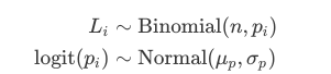
The model is not so very exotic; it is sometimes called a “logit normal” model, where the parameter for the Binomial distribution is modelled as an average constant plus some normally distributed error on the logit scale:
indeed, sampling works fine (without errors) for me, but seems to take two hours. In Stan I was able to draw three times as many samples in less than 5 min
This and that you called the sampling with the xs and ps instead of ns and xs.
Type-stability always helps to make execution of an Julia program faster. This is nothing PPL related. If the model is not type-stable the whole type inference during sampling makes the computation expensive.
We are still having a performance tips page on the todo list. @mohamed82008 , are you still working on it? Do you need some help?
Some general tips:
You should try to use multivariate distributions if possible as this will reduce allocation and computation costs. FillArrays often helps if you have a situation as in your model.
If you cannot express it using a multivariate distribution, you should use the typed syntax I proposed in one of the first posts.
Please do the following for now. I’ll included this into the PR. Sorry for the inconvenience!
using FillArrays

"""
    MvBinomialLogit(n::Vector{<:Int}, logpitp::Vector{<:Real})

A multivariate binomial logit distribution with `n` trials and logit values of `logitp`.
"""
struct MvBinomialLogit{T<:Real, I<:Int} <: DiscreteMultivariateDistribution
    n::Vector{I}
    logitp::Vector{T}
end

Distributions.length(d::MvBinomialLogit) = length(d.n)

function Distributions.logpdf(d::MvBinomialLogit{<:Real}, ks::Vector{<:Integer})
    return sum(Turing.logpdf_binomial_logit.(d.n, d.logitp, ks))
end

@model normal_logit(n, x) = begin

    n_obs = length(n)

    ## hyperparameters for varying effectgs
    ā ~ Normal(0, 0.5)
    σ_a ~ Truncated(Exponential(3), 0, Inf)

    # varying intercepts for each observation
    a ~ MvNormal(Fill(ā, n_obs), σ_a)

    x ~ MvBinomialLogit(n, a)
end
@trappmartin thank you so much for your help so far. However I can’t replicate your success so far! When I try with default settings, I get a warning, a long pause, followed by a progress bar that predicts 24 hours
this is the warning:
lbeta(x::Real, w::Real)` is deprecated, use `(logabsbeta(x, w))[1]` instead.
│   caller = logpdf_binomial_logit(::Int64, [etc]
If i set Turing.setadbackend(:reverse_diff), i get
Not implemented: convert tracked Tracker.TrackedReal{Float64} to tracked Float64
error(::String) at error.jl:33
convert(::Type{Tracker.TrackedReal{Float64}}, ::Tracker.TrackedReal{Tracker.TrackedReal{Float64}}) at real.jl:39
Could it be the versions of the packages involved?
Hi, here is an implementation that works fine on #master and should work on the latest release too. I had to remove the FillArrays bit again, don’t know why this made trouble and worked in the first place.
@mohamed82008 I think this should work with FillArrays too? Not sure why this is problematic.
using Turing
using StatsFuns

ns = fill(400, 300)

# variation in probabilities
ps = logistic.(rand(Normal(-2,0.8), 300))

xs = rand.(Binomial.(ns, ps))

struct MvBinomialLogit{T<:AbstractVector{<:Real}, I<:AbstractVector{<:Int}} <: DiscreteMultivariateDistribution
    n::I
    logitp::T
end

Distributions.length(d::MvBinomialLogit) = length(d.n)

function Distributions.logpdf(d::MvBinomialLogit, ks::AbstractVector{<:Int})
    return sum(Turing.logpdf_binomial_logit.(d.n, d.logitp, ks))
end

@model normal_logit(n, x) = begin

    n_obs = length(n)

    ## hyperparameters for varying effectgs
    b ~ Normal(0, 0.5)
    σ_a ~ Truncated(Exponential(3), 0, Inf)

    # varying intercepts for each observation
    a ~ MvNormal(fill(b, n_obs), σ_a)

    x ~ MvBinomialLogit(n, a)
end

Turing.setadbackend(:reverse_diff)
normal_logit_samples = sample(normal_logit(ns, xs), NUTS(1000, 0.8), 2000);
Not that I had to increase the number of adaptation iterations to prevent NUTS from diverging after the adaptation. I guess 1000 is unnecessary and less would work too, I didn’t play around much with it.