Multiple normal distributions in one 3D plot

Hello, I am trying to plot multiple normal distributions centered around the same mean with different variations in GLmakie. Pretty much this picture (generated in wolfram alpha):

Hopefully, also animate it by making the mean or the variances observable. Can someone please walk me through a solution?

1 Like

Hi @Mouad .

You can use something like the following:

using Distributions, GLMakie

μ3 = 0.0;
σ3 = range(1.0,10.0; length=25);
y3 = range(-10.0, 10.0; length=101);

f3 = Figure()
ax3 = Axis3(f3[1,1])
for i in σ3
    d3 = pdf.(Normal(μ3, i), y3);
    lines!(ax3, [i], y3, d3)
end
f3

Also, to specify colors along a color scale, you could add the following code:

using ColorSchemes

colors = get(ColorSchemes.viridis, range(0.0,1.0; length=length(σ3)));

where you can choose your preferred color scale substituting viridis with one of the scale names you find on the Makie color page.

Then you use add the color to the lines! command in the plotting cycle. So, the full working example could become

using Distributions, GLMakie, ColorSchemes

μ3 = 0.0; 
σ3 = range(1.0,10.0; length=25);
y3 = range(-10.0, 10.0; length=101);
colors = get(ColorSchemes.viridis, range(0.0,1.0; length=length(σ3)));

f3 = Figure()
ax3 = Axis3(f3[1,1])
for (i, σ) in enumerate(σ3)
    d3 = pdf.(Normal(μ3, σ), y3);
    lines!(ax3, [i], y3, d3, color=colors[i])
end
f3

To compare the pdfs and to convey the right information on the normal distribution, each normal pdf of mean \mu =0, and standard deviation, σ ∈ 0.5:0.25:4.0, should be represented on the interval (-3σ, 3σ), because if X \sim N(0, σ), then the probability, P(-3σ < X < 3\sigma)=\Phi(3)-\Phi(-3)=2\Phi(3)-1=0.99, where \Phi is the cdf of N(0,1). Indeed:

julia> using Distributions
julia> d = Normal(0,1);
julia> prob=2*cdf(d, 3)-1
0.9973002039367398

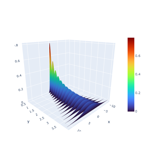
Then the graphs look as follows:

using PlotlyJS, Colors, ColorSchemes

f(x, σ; μ=0)= exp(-0.5*(x-μ)^2/σ^2)/(σ*sqrt(2π))
fig=Plot();
sigmas=0.5:0.25:4.0
n=length(sigmas)
mycolors = ColorScheme([get(ColorSchemes.turbo, t) for t in range(0, 1.0, length=n)])

for (k,σ) ∈ enumerate(sigmas)
    x= range(-3*σ, 3*σ, length=floor(Int,100*σ)) 
    addtraces!(fig, scatter3d(x=x, y=σ*ones(size(x)), z=f.(x, σ), 
                              mode="lines", name="σ: $σ",
                              line_color="#"*hex(mycolors[k]), line_width=4))
end 
relayout!(fig, width=500, height=500, #template=templates["plotly_dark"],
          scene_xaxis_range=[-3*sigmas[end], 3*sigmas[end]],
          scene_camera_eye=attr(x=1.5, y=1.5, z=0.7), font_size=11, 
          )
display(fig)

Npdfs-lines

or as surfaces:
Npdfs-surfs

2 Likes