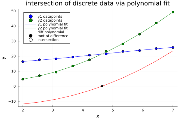
Some example code for computing the intersection of curves from discrete data points using polynomial fits.
This code blocks creates some artificial data.
using Polynomials, Plots

# two functions that intersect on an interval (a,b)
f1(x) = 2x + 12
f2(x) = x^2

(a,b) = (2,7)   # the interval of interest
n = 10           # number of data points
ynoise = 0.3     # noise level, absolute

# create some noisy data from those two functions
x = range(a, b, length=n)
y1 = f1.(x) + ynoise*randn(n)
y2 = f2.(x) + ynoise*randn(n)
This code block computes polynomial fits, finds the intersection point as a root of the difference polynomial, and plots the results To see how it works and the types it generates, you might want to step through it line by line at the REPL.
y1poly = fit(x,y1, 3)               # make 3rd order polynomial fit to y1 data
y2poly = fit(x,y2, 3)               # same for y2
ydiffpoly = y2poly - y1poly         # compute difference of y2,y1 polynomials

xroots = roots(ydiffpoly)           # find roots of difference polynomial
j = findall(z -> a ≤ z ≤ b, xroots) # find the indices of the roots with interval (a,b)
xr = xroots[j[1]]                   # select the first root in the interval
yr = y1poly(xr)                     # compute y value at intersection point

scatter(x, y1, label="y1 datapoints", mc=:blue)
scatter!(x, y2, label="y2 datapoints", mc=:green)

plot!(x, y1poly.(x), label="y1 polynomial fit", lc=:blue)
plot!(x, y2poly.(x), label="y2 polynomial fit", lc=:green)
plot!(x, ydiffpoly.(x), label="diff polynomial", lc=:red)

scatter!(x, y1, label="", mc=:blue)
scatter!(x, y2, label="", mc=:green)

scatter!([xr], [ydiffpoly(xr)], label="root of difference", mc=:black)
scatter!([xr], [yr], label="intersection", mc=:white)
plot!(xl="x", yl="y", legend=:topleft)
plot!(title="intersection of discrete data via polynomial fit")
