Lining up zeros on plot with 2 y axes

Hi there,

I am plotting 2 different datasets on the same plot, but using different scaled y axes, using the following code:

plot(ShiSimpleSolV, idxs = [circ_sys.MV.q])

plot!(twinx(), ShiSimpleSolV, idxs = [circ_sys.MV.Δp], linecolor=:red)

which produces:
image

I was wondering if there was a way to line up the zeros so they are at the same height? I want to try to show how the blue line only increases when the red line is below zero.

Also is there a way to turn off the second x axis label?

Thank you!

Since you seem to be using the DifferentialEquations.jl Plots’ recipes, you could try the example below (where sol is the diffeq solution):

using Plots; gr(dpi=600)

# Assumes that 1st curve has both + and - values
a, b, c, d = extrema(sol[1,:])..., extrema(sol[2,:])...
α = -b/a
c * d ≥ 0 && (c = -d/α)
β = -d/c
α > β ? d = -α*c : c = -d/α

plot(sol, idxs=1, ylims=(a,b), c=:blue, framestyle=:zerolines, ylabel="u1", yguidefontcolor=:blue, legend=:topright)

plot!(twinx(), sol, idxs=2, ylims=(c,d), c=:red, grid=true, xlabel="", ylabel="u2", yguidefontcolor=:red, legend=:bottomleft)

Plot example:

With the same concept as @rafael.guerra 's answer. But a much more verbose version:

function matchpratio(lims1, lims2, p = 0.0)
    lo, hi = lims1
    lo >= hi && error("lims must be ordered")
    newlo = min(p, lo)
    newhi = max(p, hi)
    pratio = (p - newlo) / (newhi - newlo)
    lo2, hi2 = lims2
    lo2 >= hi2 && error("lims must be ordered")
    newlo2 = min(p, lo2)
    newhi2 = max(p, hi2)
    pratio2 = (p - newlo2) / (newhi2 - newlo2)
    if pratio2 > pratio
        newhi2 = (p - newlo2) / pratio
    else
        newlo2 = newhi2 - (newhi2 - p) / (1 - pratio)
    end
    if any(isinf, (newlo, newhi, newlo2, newhi2))
        a,b = matchpratio(lims2, lims1, p)
        return (b,a)
    end
    return ((newlo, newhi), (newlo2, newhi2))
end

and now:

julia> y1 = cumsum(rand(10));

julia> y2 = cumsum(rand(10)) .- 3;

julia> l1, l2 = matchpratio(extrema(y1), extrema(y2))
((-5.927414300344668, 6.473046090935813), (-2.743430915758225, 2.9959698892599125))

julia> plt = plot(y1; line = (:green, :step), ylim=l1);

julia> plot!(twinx(), y2; line = (:red, :step), ylim=l2)

and the function matchpratio works for other points of interest using the third argument.

That’s great thank you so much, it now looks like this:


I was wondering if there was a way to add in the markers for the u1 y axis while still having the x axis at the zero line?
I got rid of the framestyle=:zerolines in the first plot(), which gave this:

Which is still fine but ideally the black x-axis line would still be at the zero line.

Also, is there a way of having the legends in the same box?

Thanks again?

I do not understand this requirement, could you ellaborate?

Yes, you can check the edited code:

plot(sol, idxs=1, ylims=(a,b), c=:blue, framestyle=:zerolines, ylabel="u1", yguidefontcolor=:blue, legend=:topright)
plot!((0, NaN), c=:red, label="u2(t)")
plot!(twinx(), sol, idxs=2, ylims=(c,d), c=:red, grid=true, xlabel="", ylabel="u2", yguidefontcolor=:red, label="")

which plots:

Hi sorry, hopefully I can explain a bit better. When I run the following code (your example applied to my data)

a, b, c, d = extrema(sol[circ_sys.MV.Δp])..., extrema(sol[circ_sys.MV.q])...
α = -b/a
c * d ≥ 0 && (c = -d/α)
β = -d/c
α > β ? d = -α*c : c = -d/α

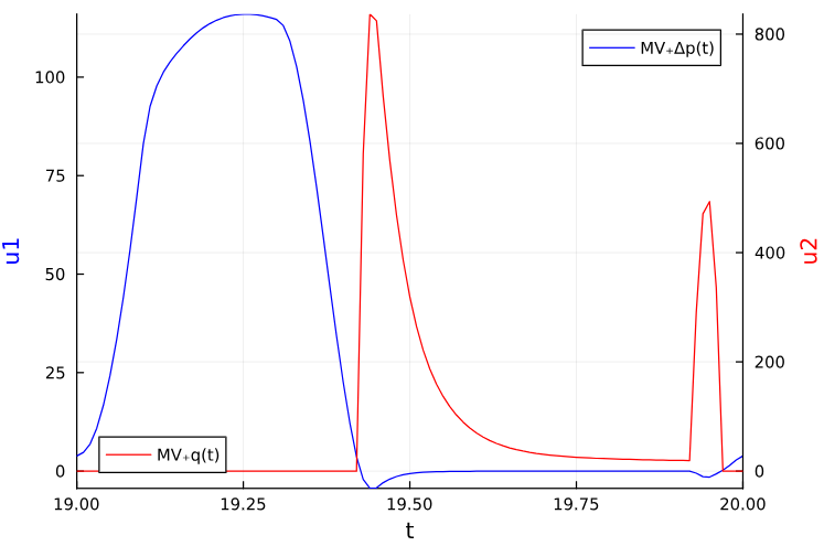
plot(sol, idxs=circ_sys.MV.Δp, ylims=(a,b), c=:blue, framestyle=:zerolines, ylabel="u1", yguidefontcolor=:blue, legend=:topright)

plot!(twinx(), sol, idxs=circ_sys.MV.q, ylims=(c,d), c=:red, grid=true, xlabel="", ylabel="u2", yguidefontcolor=:red, legend=:bottomleft)

I get the following graph

Here the black line for the x-axis is where I want it to be (at y=0), but I would like to add a black line at the u1 y-axis. In order to do this, I tried to get rid of the framestyle=:zerolines parameter in the first plot() command, resulting in the following plot commands:

plot(sol, idxs=circ_sys.MV.Δp, ylims=(a,b), c=:blue, ylabel="u1", yguidefontcolor=:blue, legend=:topright)

plot!(twinx(), sol, idxs=circ_sys.MV.q, ylims=(c,d), c=:red, grid=true, xlabel="", ylabel="u2", yguidefontcolor=:red, legend=:bottomleft)

And gives the following graph:

This has the black line at the u1 y-axis that I want, however the the black x-axis is no longer at the y=0 line.

Is there a way of resolving this? I see that in the plot you have as an example, this black y-axis line is there, so I don’t know why this is not working for me.

Thanks again

Ah, OK, that is because my plot starts at t=0.

A simple fix is to add a vertical line at the initial time t₀ of your simulation.

vline!([t₀], c=:black)

With more labor, you could add the xticks too.

1 Like

Thanks so much for all your help!

1 Like