Is There Package or Method to Calculate Certain Area in Julia (symbolically with SymPy)?

[Freya_the_Goddess]

Hi all,

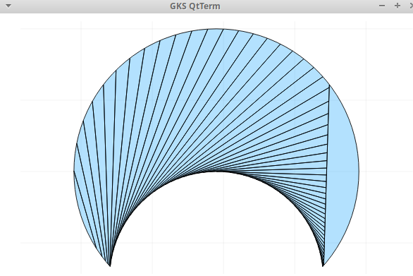
there are two circles, one is bigger than the other, and overlapping a bit, I want to know could Julia help to calculate the bigger circle shaded area? Maybe this is geometry problem. But it is on Calculus book.

This is the solution:

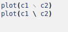
I am using Latex to draw it, I can’t hardly plot it with Julia, too difficult:

\documentclass[12pt]{article}
\usepackage{tikz}
\usetikzlibrary{decorations.pathreplacing}
\usetikzlibrary {calc}

\newcommand{\MarkRightAngle}[4][.3cm]% #1=size (optional), #2-#4 three points: \angle #2#3#4
{\coordinate (tempa) at ($(#3)!#1!(#2)$);
	\coordinate (tempb) at ($(#3)!#1!(#4)$);
	\coordinate (tempc) at ($(tempa)!0.5!(tempb)$);%midpoint
	\draw (tempa) -- ($(#3)!2!(tempc)$) -- (tempb);
}

\begin{document}
	\begin{tikzpicture}[scale=1,>=latex,x=1cm,y=0.8cm]
		
		\draw[fill=blue!7] (0,0) ellipse (4 and 4);% a circle 
		\draw[fill=blue!7] (-4,0) arc (180:360:4 and 4);% left half of the circle starting at (-4,0) from 180 to 360
		\draw[fill=white!7] (0,-3) ellipse (3 and 3);% a circle 
		
		\draw (0,0.2) node {$A$};
		\draw (0,-3.6) node {$C$};
		\draw (-3.5,-3.1) node {$D$};	
		\draw (3.5,-3.1) node {$B$};
		\draw (1.5,-3.2) node {$a$};	
		
		% Create right angle
		\coordinate (A) at (0,0);
		\coordinate (E) at (1.6,-1.4);
		\coordinate (C) at (0,-3);
		\MarkRightAngle{A}{E}{C}
		
		\draw[dashed] (0,-3) -- (1.6,-1.4);
		\draw[-,thick] (0,0) -- (-3,-2.7) node[left, midway]  {\footnotesize $b$};
		\draw[-,thick] (0,0) -- (3,-2.7) node[right, midway]  {\footnotesize $E$};
		\draw[-,thick] (0,0) -- (0,-3) node[left, midway]  {\footnotesize $a$};
		\draw[-,thick] (-3,-2.7) -- (0,-3);
		\draw[-,thick] (3,-2.7) -- (0,-3);
		
	\end{tikzpicture}
\end{document}

The question is:
If I plot it with Julia, two circles with certain radius and center, can I compute the certain area that is not intersected with other geometry object like the solution above?

[DanielVandH]

Never used it, but you could take a look at GitHub - mancellin/PolygonArea.jl: A claimless Julia library to compute the area of unions and intersections of polygons. I don’t imagine you’d be able to do much here symbolically, though.

[Freya_the_Goddess]

Alright thanks for this, I will check it out

[Freya_the_Goddess]

The package can draw intersection and union, but not setminus…

using PolygonArea, Plots

r = rectangle((0.0, 0.0), (1.0, 1.0))

c1 = circle((0.9, 1.5), 1.5, 100)  # Actually, a regular 100-gon
c2 = circle((0.9, 3), 2, 100)  # Actually, a regular 100-gon

cinter = c1 ∩ c2
#a = area(c1 ∩ c2)
#println("area =   ", a)
plot(c2)
plot!(c1, color=:green)

#plot(c1 ∖ c2) does not work

[rocco_sprmnt21]

To draw the figure you could use this package, although perhaps it needs to be tuned better for a better definition.
To have a symbolic solution, either do it by hand or try with GPT v5

using ImplicitEquations, Plots
f(x,y) = (x-0.9)^2+(y-1.5)^2-1.5^2
g(x,y) = (x-0.9)^2+(y-3.)^2-2.0^2

plot((g ≦ 0) & (f ≫ 0) , fc=:black, widen=false, aspect_ratio=:equal)   

this is the figure obtained. Maybe someone knows how to make it better.

[rocco_sprmnt21]

i tried kinda PLAYING with sympy.

using SymPy

@syms x y

julia> f(x,y) = (x-9//10)^2+(y-3//2)^2-(3//2)^2
f (generic function with 2 methods)

julia> g(x,y) = (x-9//10)^2+(y-3)^2-2^2
g (generic function with 1 method)

julia> ((x1,y1),(x2,y2))=solve([f(x,y) , g(x,y)], x, y)
2-element Vector{Tuple{Sym, Sym}}:
 (9/10 - 2*sqrt(5)/3, 5/3)
 (9/10 + 2*sqrt(5)/3, 5/3)

julia> ft(x,y) = (x)^2+(y+5//3-3//2)^2-(3//2)^2
ft (generic function with 1 method)

julia> gt(x,y) = (x)^2+(y+5//3-3)^2-2^2
gt (generic function with 1 method)

julia> ((x1,y1),(x2,y2))=solve([ft(x,y) , gt(x,y)], x, y)
2-element Vector{Tuple{Sym, Sym}}:
 (-2*sqrt(5)/3, 0)
 (2*sqrt(5)/3, 0)

julia> nscf(x),pscf(x)=solve(ft(x,y),y)
2-element Vector{Sym}:
 -sqrt(9 - 4*x^2)/2 - 1/6
  sqrt(9 - 4*x^2)/2 - 1/6

julia> S1=integrate(pscf(x), x1,x2)
             ⎛4⋅√5⎞
       9⋅asin⎜────⎟
  √5         ⎝ 9  ⎠
- ── + ────────────
  9         4

julia> nscg(x),pscg(x)=solve(gt(x,y),y)
2-element Vector{Sym}:
 4/3 - sqrt(4 - x^2)
 sqrt(4 - x^2) + 4/3

julia> S2=integrate(nscg(x), x1,x2)
        ⎛√5⎞   8⋅√5
- 4⋅asin⎜──⎟ + ────
        ⎝3 ⎠    9

julia> Sym(π)*4- (S1-S2)
                     ⎛4⋅√5⎞
               9⋅asin⎜────⎟
        ⎛√5⎞         ⎝ 9  ⎠
- 4⋅asin⎜──⎟ - ──────────── + √5 + 4⋅π
        ⎝3 ⎠        4

[Freya_the_Goddess]

Very beautiful @rocco_sprmnt21 . This is why I find enjoyment learning Mathematics and sharing here in this discourse. The experts help beginner like me a lot.

[rocco_sprmnt21]

I too (not being a real expert, like many others in this forum) find it interesting to follow the discussions and, when possible, participate.

I would like to add an observation. Maybe a bit fussy, but that might be why symbolic solving with SymPy functions doesn’t come “easy”.

The practical observation is that the result shown in the book is valid only for a/b >=1/2.

For a/b<1/2 the gray surface is always S(a/b=1/2)

An additional observation is that it would be nice to be able to add assumptions (constraints?) in order to “oblige” the SymPy functions to give only the “physically/geometrically” expected solutions.

[rocco_sprmnt21]

Without losing generality, the figures can be translated into a reference of Cartesian axes, so as to have the center of the circle of radius b at the origin O of the axes.
Similarly, to make life easier for SymPy, you can scale everything by a factor b, so that b=>1 to a=>a/b.
So the transformations that serve to symbolically solve the problem are the following.

julia> using SymPy

julia> @syms x
(x,)

julia> @vars a y positive=true
(a, y)

julia> ft(x,y) = (x-a)^2+(y)^2-a^2
ft (generic function with 1 method)

julia> gt(x,y) = (x)^2+(y)^2-1
gt (generic function with 1 method)

julia> (x1,y1)=solve([ft(x,y) , gt(x,y)], x, y)[1]
(1/(2*a), sqrt(2*a - 1)*sqrt(2*a + 1)/(2*a))

julia> nscf(x),pscf(x)=solve(ft(x,y),y)
2-element Vector{Sym}:
 -sqrt(x*(2*a - x))
  sqrt(x*(2*a - x))

julia> S1=integrate(expand(pscf(x)), (x, 0,x1)) # using pscf(x) whitout expand give a messy formula
       ⎛      1 ⎞
       ⎜-a + ───⎟
 2     ⎜     2⋅a⎟
a ⋅asin⎜────────⎟      2        __________
       ⎝   a    ⎠   π⋅a        ╱      1    ⎛  a    1 ⎞
───────────────── + ──── +    ╱  1 - ──── ⋅⎜- ─ + ───⎟
        2            4       ╱          2  ⎝  2   4⋅a⎠
                           ╲╱        4⋅a

julia> nscg(x),pscg(x)=solve(gt(x,y),y)
2-element Vector{Sym}:
 -sqrt(1 - x^2)
  sqrt(1 - x^2)

julia> S2=integrate(pscg(x), (x, x1,1))
                       __________
                      ╱      1
      ⎛ 1 ⎞          ╱  1 - ────
  asin⎜───⎟         ╱          2
      ⎝2⋅a⎠   π   ╲╱        4⋅a
- ───────── + ─ - ───────────────
      2       4         4⋅a

I enclose the analogous operations done by hand.
With a little patience it can be verified that the two results are equivalent

[Freya_the_Goddess]

That is a very nice observation knowing the result only valid for a/b >= 1/2.

We will always need assumptions and constraints then, because if not limited then the solution is boundless.

[mancellin]

Hi, I’m the author of PolygonArea.jl. Thank you for considering using it!

Actually set difference has been implemented but with the backslash \ operator as I wasn’t aware of \setminus (sorry for the lack of documentation).

Anyway, the implementation of PolygonArea is dreadfully inefficient for concave shapes with many edges, such as your c1 \ c2.
But if you only need the area, maybe you could do instead

area(c1) - area(c1 ∩ c2)

that should work fine.

[Freya_the_Goddess]

Hi @mancellin ,

thanks for the package, it is really amazing and useful for students like me.

I want to straighten out that the mistake is on the character, I type this:

plot(c1 ∖ c2)

but the backlash is from copy paste from Julia Documentation, I should have type backlash directly from keyboard, notice this when I see it from Mousepad / Notepad of Linux:

The above won’t work. but below will work.

My mistake.

This code works:

# https://discourse.julialang.org/t/is-there-package-or-method-to-calculate-certain-area-in-julia-symbolically-with-sympy/99751/4

using PolygonArea, Plots

r = rectangle((0.0, 0.0), (1.0, 1.0))

c1 = circle((0.9, 1.5), 1.5, 100)  # Actually, a regular 100-gon
c2 = circle((0.9, 3), 2, 100)  # Actually, a regular 100-gon

cinter = c1 ∩ c2
#a = area(c1 ∩ c2)
#println("area =   ", a)
#plot(c2)
#plot!(c1, color=:green)


plot(c2 \ c1) 

I love trying Julia and its packages, it is amazing for people around the world to learn Mathematics with Computer Science at one time.

[Freya_the_Goddess]

This is something that I want to ask:

If we can get the \theta and \phi from angle DCB and angle DAB in terms of \arccos and \arcsin from the solution above, Why the solution suggest that \theta and \phi are in radians?

Btw,

b = radius of big circle
a = radius of small circle

The small circle perimeter (North perimeter) hit the center of the big circle.

[rocco_sprmnt21]

I don’t know how pertinent this is to Julia and I’m not sure of the author’s motivation in preferring the use of radians to degrees.
I would think that a good reason could be the greater simplicity of the formulas, in the case of the use of radians.
For example a famous limit of analysis [lim(sin(x)/x) when x->0] = 1 only if x is measured in radians.