Euler Equation Iteration to solve an Optimization problem

Albert_Zevelev · July 12, 2022, 11:49pm

I would like to solve a simple/routine economics problem with Euler Equation Iteration.
The following code works well:

using Interpolations, Plots, LinearAlgebra
#
PolyBasis(K)     = [ones(size(K)) K K.^2] 
PolyGetCoef(K,Y) = PolyBasis(K) \ Y
#
β = 0.99; α = 0.36; z=1.0; γ = 2.0; δ = 1.0;
s_ss = ( (1/β -1 +δ) / (α*z) )^(1/(α-1)); 
f(s1; z=z,α=α,δ=δ)      =   z*(s1^α)     +(1-δ)*s1
fprime(s1; z=z,α=α,δ=δ) = α*z*(s1^(α-1)) +(1-δ)
#
S1 = [range(0.75*s_ss, 1.25*s_ss,length=100);]
T1(s1,c1) = f(s1) - c1
Π10 = [ f(s1) - δ*s1  for s1 in S1] 
EE1(s1,sp1,cp1; β=β,γ=γ) = (cp1) * ((β*fprime(sp1))^(-1/γ))
#EE1(s1,sp1,cp1; β=β,γ=γ) = min((cp1) * ((β*fprime(sp1))^(-1/γ)), f(s1))
#
@inline function FPI_EE(S1, Π1; k_max=100, tol=0.001)
    dist = 10.0; k=1;
    @inbounds while(dist > tol && k<=k_max) 
        println(k)
        #
        b  = PolyGetCoef(S1, Π1)
        c1 = PolyBasis(S1)*b # ≈Π1
        sp1 = T1.(S1, c1)
        cp1 = PolyBasis(sp1)*b
        Πp1 = EE1.(S1, sp1, cp1)
        dist = norm(Π1 - Πp1) 
        k += 1
        Π1 = Πp1
    end 
    return Π1
end
@time Pol_EE = FPI_EE(S1, Π10; k_max=5000)
plot(S1, Pol_EE, legend=:false)

Everything works well. But it stops converging when γ<1.78.

Does anyone know why? Or how to fix this?
Here is the solution (policy function) for a grid of γ:

nicolas · July 13, 2022, 3:19pm

I think your grid for K is too narrow. For γ=1.7, the solution converges when changing the line
S1 = [range(0.75 * s_ss, 1.25 * s_ss, length=100);]
to
S1 = [range(0.75 * s_ss, 3 * s_ss, length=100);]

Albert_Zevelev · July 13, 2022, 3:28pm

I’ll try it later.
My goal is to solve the case gamma =1 so I can compare to closed form.
Does that case still work?

nicolas · July 13, 2022, 3:46pm

γ=1 seems a hard one. I’ve tried some things including different starting guesses for Π10 and I keep getting negative values or cycles. If you actually know the solution you think you should get, you can try it as initial guess for Π10, or something very close, and see whether at least the fixed point is attracting. Otherwise you would have to solve it in a different way I’m afraid.

Albert_Zevelev · July 13, 2022, 3:49pm

It’s the usual closed form solution to the NGM w log utility:

I tried using it as a guess yesterday without luck

Albert_Zevelev · July 13, 2022, 6:25pm

I tried a different version w/ a different approx & starting w/ a guess equal to the closed form solution does converge:

using Interpolations, Plots, LinearAlgebra
@inline approx(gr, val0) = LinearInterpolation(gr, val0, extrapolation_bc = Line())
#
β = 0.99; α = 0.36; z=1.0; δ = 1.0; γ = 1.0;
f(s1; z=z,α=α,δ=δ)      =   z*(s1^α)     +(1-δ)*s1
fprime(s1; z=z,α=α,δ=δ) = α*z*(s1^(α-1)) +(1-δ)
c_CF(s1; z=z,α=α,β=β) = (1-α*β)*z*(s1^α)
#
s_ss = ( (1/β -1 +δ) / (α*z) )^(1/(α-1)) 
c_ss = f(s_ss) -s_ss
#
S1 = [range(0.025*s_ss, 3*s_ss,length=1000);]
T1(s1,c1) = f(s1) - c1
EE1(s1,sp1,cp1; β=β,γ=γ) = (cp1) * ((β*fprime(sp1))^(-1/γ))
#
@inline function FPI_EE(S1, Π1; k_max=100, tol=0.001)
    dist = 10.0; k=1;
    @inbounds while(dist > tol && k<=k_max) 
        println(k)
        #
        Πh1 = approx((S1), Π1)
        sp1 = T1.(S1, Π1)
        cp1 = Πh1.(sp1)
        Πp1 = EE1.(S1,sp1,cp1)    # Π Improvement/Update
        #
        plot!(S1, Πp1) |> display
        #k % 50 ==0 ? plot!(S, Πp) |> display : nothing  
        dist = norm(Π1 - Πp1) 
        k += 1
        Π1 = Πp1
    end 
    return Π1
end
Π10 = [ c_CF(s1)   for s1 in S1] 
#
plot(S1, f, legend=:false)
plot!(S1, Π10)
plot!([s_ss],  seriestype = :vline, lab="", color="grey")
plot!([c_ss],  seriestype = :hline, lab="", color="grey")
@time Pol_EE = FPI_EE(S1, Π10; k_max=200)

However if I start slightly below/above the correct solution:
Π10 = [ .99*c_CF(s1) for s1 in S1]
it blows up.

BTW, part of the reason is the for Kp \geq 0 we need c \leq f(K).
I can change the EulerEquation function to incorporate this:
EE1(s1,sp1,cp1; β=β,γ=γ) = min((cp1) * ((β*fprime(sp1))^(-1/γ)), f(s1))
Now I don’t have complex number problems, but it still doesn’t converge…

nicolas · July 13, 2022, 10:49pm

Ok, so your map is clearly not a contraction. This is required to guarantee convergence. Luckily SpeedMapping can still work for expanding maps as long as it does not diverge too fast to infeasible points. So your change to the Euler equation is helpful.

function FPI_EE_map(Πp1, S1, Π1)
    Πh1 = approx((S1), Π1)
    sp1 = T1.(S1, Π1)
    cp1 = Πh1.(sp1)
    Πp1 .= EE1.(S1, sp1, cp1)    # Π Improvement/Update
end

badΠ10 = [0.9c_CF(s1) for s1 in S1]
trueΠ10 = [c_CF(s1) for s1 in S1]

using SpeedMapping
res = speedmapping(badΠ10; (m!)=(Πp1, Π1) -> FPI_EE_map(Πp1, S1, Π1)).minimizer

norm(res - trueΠ10)

Which gives

julia> norm(res - trueΠ10)
1.1706510230617607e-6

Albert_Zevelev · July 13, 2022, 11:07pm

It works (robustly for \gamma>.75), I wish I understood why

Albert_Zevelev · July 13, 2022, 11:29pm

PS: I’ve been interested in creating a generic/composable package for Fixed Point Iteration (FPI) methods & it looks like SpeedMapping.jl can be super-helpful.

Here is a generic 1-state/1-choice discrete-time/deterministic problem:
(I can make it more generic…)

Here is my interpretation of the Algorithms in Coleman, Lyon, Maliar, Maliar:

Here are the functional forms that need to be plugged in:

Are you interested in also working on creating generic FPI solvers for dynamic optimization problems in Julia?
The world would be a much better place…

nicolas · July 14, 2022, 12:55pm

I’m happy it works. It does for many cases, although I can’t guarantee it always will. Some arbitrary choices must be made as to what the right direction is (thinking about it, I could give more freedom to users on this. I will think some more).

Albert_Zevelev · July 14, 2022, 2:12pm

Initially I thought SpeedMapping.jl only speeds up function iteration. It turns out it also increases the probability the iteration will converge (based on my usage).

This is important for economics bc there is a large class of Fixed Point Iteration methods for solving dynamic optimization problems.

A few of these FPI methods (like VFI & extensions) iterate on a contraction, so they are guaranteed to converge
1: from any guess
2: to the unique fixed point

Many other FPI methods in general are not guaranteed to converge, from any guess, to a unique fixed point. These other methods (Euler iteration etc) don’t always work, but when they do, they often outperform VFI by a lot.
Your package increases the probability these other FPI methods will converge which the world needs to know.

To clarify: your package doesn’t just do FP acceleration, it increases the probability of convergence.

nicolas · July 14, 2022, 11:34pm

I agree. This could be very helpful for many domains (for instance, I’ve had a recent discussion with a quantum physicist who needed the package adapted to his needs).

I don’t think much exists in Julia except Anderson Acceleration in NLsolve.jl and N-GMRES and O-ACCEL in Optim.jl.

While developing SpeedMapping, I tried comparing its performance to the best competition I could find, so I already wrote in Julia:

Zhou, H., Alexander, D. and Lange, K. (2011). A quasi-Newton acceleration for high-
dimensional optimization algorithms. Statistics and computing 21: 261-273.

and

Henderson, N. and Varadhan, R. (2019). Damped Anderson acceleration with restarts
and monotonicity control for accelerating EM and EM-like algorithms. Journal of
Computational and Graphical Statistics 28: 834-846.

Recently, I’ve found many others. The interest in Anderson Acceleration has been growing steadily in recent years (to non-smooth maps, to domain-specific problems, etc). Choosing the right ones is the interesting part.

SpeedMapping is fairly new; I presented it at JuliaCon last year. Some problems probably still need to be ironed out, but the only way to find them at this point is for people to try it and complain back to me. So I’d happily include it in a generic FPI package. Let’s talk some more.

ChrisRackauckas · July 15, 2022, 9:58am

And one baked into the ODE solvers

Albert_Zevelev · July 16, 2022, 2:55am

Are you aware of this package:

It has 8 algorithms for fixed point acceleration.

Would be awesome if all the algorithms were together in one good well maintained package

nicolas · July 17, 2022, 12:49pm

Ah yes I think I saw that one too a while ago but forgot about it. I think that’s a great start and new algorithms can surely be incorporated.

Albert_Zevelev · July 21, 2022, 6:16pm

I’d like to apply your package to a problem with 2-state variables & 2 -choice variables.
\max_{c_t, b_{t+1}, i_{t}, h_{t+1}} \sum_{t=0}^{\infty} \beta^t u(c_t, h_t)
b_{t+1}= Rb_t -c_t -i_t -\phi(i_{t})
h_{t+1} = (1-\delta)h_{t} + i_{t}
Let: u(c,h) = \alpha ln(c) + \gamma ln(h) and \phi(i) = \frac{\theta}{2} (i)^2

Two state variables: b_{t+1}, h_{t+1} we are given b_0, h_0
Two choice variables: c_t, i_t
The equations that need to be solved: (4 equations in 4 variables)
c_{t} = (R\beta)^{-1} c_{t+1}
i_{t} = \frac{\gamma}{\alpha R \theta} \frac{c_{t+1}}{h_{t+1}} +\frac{1-\delta}{R} i_{t+1} - \frac{r+\delta}{R \theta}
b_{t+1}= Rb_t -c_t -i_t -\phi(i_{t})
h_{t+1} = (1-\delta)h_{t} + i_{t}

Note:
h_{t+1} \geq 0 \Rightarrow i_{t} \geq -(1-\delta)h_{t}
b_{t+1} \geq -\eta \Rightarrow c_t +i_t +\phi(i_{t}) \leq Rb_t +\eta {natural borrowing constraint}
c_{t} \geq 0 \Rightarrow i_t +\phi(i_{t}) \leq Rb_t - b_{t+1} \leq Rb_t +\eta

Maximum consumption if you sell all capital & borrow to limit:
c_{t} = Rb_t -b_{t+1} -i_t -\phi(i_{t})
c_{t} = Rb_t +\eta +(1-\delta)h_{t}- \frac{\theta}{2} ((1-\delta)h_{t})^2

Thus:
-(1-\delta)h_{t} \leq i_{t} \leq \frac{1}{\theta} (-1+ \sqrt{1+2\theta (Rb_t +\eta)} )
0 \leq c_{t} \leq Rb_t +\eta +(1-\delta)h_{t}- \frac{\theta}{2} ((1-\delta)h_{t})^2

Now Euler Iteration code: c_{1t}\equiv c_{t}, c_{2t}\equiv i_{t}, s_{1t}\equiv b_{t}, s_{2t}\equiv h_{t}

#
r = 0.05; R = (1+r); θ = 1.00; δ = 0.10; α = 0.50; γ = 0.50; β=1/R; 
ϕ(c2;θ=θ) = .5*θ*(c2^2)
#
S1 = [(.01 : .01 : 2.5);] 
S2 = [(.01 : .01 : 2.5);]    #S = [S1 S2] 
#
T1(s1,s2,c1,c2; R=R) = R*s1 -c1 -c2 -ϕ(c2)
T2(s1,s2,c1,c2; δ=δ) = (1-δ)*s2 +c2
#
η=0.0
c1_EE1(s1,s2,s1p,s2p,c1p,c2p; R=R,β=β) = c1p*((R*β)^(-1))
c1_min(s1,s2) = 0.00001      # c1 >= 0.0
c1_max(s1,s2;R=R,δ=δ,η=η) = R*s1 +η +(1-δ)*s2 - ϕ((1-δ)*s2) # c1 <= R*(s1) + z - η => s1p>=0
#
c2_EE2(s1,s2,s1p,s2p,c1p,c2p; R=R,γ=γ,α=α,θ=θ,δ=δ) = (γ/(α*R*θ))*(c1p/s2p) +((1-δ)/R)*c2p -((R-1+δ)/(R*θ))
c2_min(s1,s2) = -(1-δ)*s2
c2_max(s1,s2;R=R,θ=θ,η=η) = (1/θ)*(-1 + sqrt(1+2*θ*(R*s1+η)))
#
EE1(s1,s2,s1p,s2p,c1p,c2p) = clamp(c1_EE1(s1,s2,s1p,s2p,c1p,c2p), c1_min(s1,s2), c1_max(s1,s2)) # clamp(x, lo, hi) 
EE2(s1,s2,s1p,s2p,c1p,c2p) = clamp(c2_EE2(s1,s2,s1p,s2p,c1p,c2p), c2_min(s1,s2), c2_max(s1,s2)) # clamp(x, lo, hi) 
#
function FPI_EE_map!(Π1p, Π2p, Π1, Π2, S1, S2)
    #
    Π1h = approx((S1, S2), Π1)
    Π2h = approx((S1, S2), Π2)
    S1p = [T1(S1[j], S2[k], Π1[j,k], Π2[j,k]) for j in eachindex(S1), k in eachindex(S2)]
    S2p = [T2(S1[j], S2[k], Π1[j,k], Π2[j,k]) for j in eachindex(S1), k in eachindex(S2)]
    C1p = [Π1h(S1p[j,k], S2p[j,k]) for j in eachindex(S1), k in eachindex(S2)]
    C2p = [Π2h(S1p[j,k], S2p[j,k]) for j in eachindex(S1), k in eachindex(S2)]
    Π1p .= [EE1(S1[j], S2[j], S1p[j,k], S2p[j,k], C1p[j,k], C2p[j,k]) for j in eachindex(S1), k in eachindex(S2)]
    Π2p .= [EE2(S1[j], S2[j], S1p[j,k], S2p[j,k], C1p[j,k], C2p[j,k]) for j in eachindex(S1), k in eachindex(S2)]
end
#
Π10 = [.1 for s1 in S1, s2 in S2] #
Π20 = [.1 for s1 in S1, s2 in S2] #
#
res = speedmapping(Π10,Π20; (m!)=(Π1p, Π2p, Π1, Π2) -> FPI_EE_map!(Π1p, Π2p, Π1, Π2, S1, S2))

Is it possible to do this with your package?

Albert_Zevelev · July 27, 2022, 12:07am

A cleaner & simpler example of a 2-state/2-choice problem is the Uzawa-Lucas model.

A special case (full depreciation & log utility) has a closed form solution:

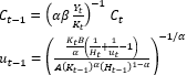
The Euler equations if \gamma =0 (no externality)

Now in Julia

using Interpolations, Plots, LinearAlgebra, SpeedMapping
@inline approx(gr, val0) = LinearInterpolation(gr, val0, extrapolation_bc = Line())
#
α=.33; β=.97; #σ=1;δ=0;A=1.0; 
F(K,H,u;α=α) = (K^α)*(u^(1-α))*(H^(1-α))
#
γ=0.0;
ū=((1-α)*(1-β))/(1-α+β*γ)
B= 1/(1.0 - ū) + .02
#B= 1/(1.0 - ū) - .02
#B= 1/(1.0 - ū) 
#
S1 = [(.01 : .01 : 1.0);] 
S2 = [(.01 : .01 : 1.0);]    #S = [S1 S2]  PolyBasis(S1, S2)
#
T1(s1,s2,c1,c2) = F(s1,s2,c2) -c1
T2(s1,s2,c1,c2; B=B) = B*(1-c2)*s2
#
c1_EE1(s1,s2,s1p,s2p,c1p,c2p; α=α,β=β) = c1p*((β*α*(F(s1p,s2p,c2p)/s1p))^(-1))
c1_min(s1,s2) = 0.00001      # c1 >= 0.0
c1_max(s1,s2) = F(s1,s2,1.0) # c1 <=
#
c2_EE2(s1,s2,s1p,s2p,c1p,c2p;B=B,α=α) = ((s1p*B/α)*(1/s2p +1/c2p -1)/((s1^α)*(s2^(1-α))))^(-1/α)
c2_min(s1,s2) = 0.0
c2_max(s1,s2) = 1.0
#
EE1(s1,s2,s1p,s2p,c1p,c2p) = clamp(c1_EE1(s1,s2,s1p,s2p,c1p,c2p), c1_min(s1,s2), c1_max(s1,s2))
EE2(s1,s2,s1p,s2p,c1p,c2p) = clamp(c2_EE2(s1,s2,s1p,s2p,c1p,c2p), c2_min(s1,s2), c2_max(s1,s2))
#
Π10 = [(1-α*β)*F(s1,s2,ū) for s1 in S1, s2 in S2] #
Π20 = [ū for s1 in S1, s2 in S2] #
#
function FPI_EE_map!(Π1p, Π2p, Π1, Π2, S1, S2)
    #
    Π1h = approx((S1, S2), Π1)
    Π2h = approx((S1, S2), Π2)
    S1p = [T1(S1[j], S2[k], Π1[j,k], Π2[j,k]) for j in eachindex(S1), k in eachindex(S2)]
    S2p = [T2(S1[j], S2[k], Π1[j,k], Π2[j,k]) for j in eachindex(S1), k in eachindex(S2)]
    C1p = [Π1h(S1p[j,k], S2p[j,k]) for j in eachindex(S1), k in eachindex(S2)]
    C2p = [Π2h(S1p[j,k], S2p[j,k]) for j in eachindex(S1), k in eachindex(S2)]
    Π1p .= [EE1(S1[j], S2[j], S1p[j,k], S2p[j,k], C1p[j,k], C2p[j,k]) for j in eachindex(S1), k in eachindex(S2)]
    Π2p .= [EE2(S1[j], S2[j], S1p[j,k], S2p[j,k], C1p[j,k], C2p[j,k]) for j in eachindex(S1), k in eachindex(S2)]
end
#res = speedmapping(Π10,Π20; (m!)=(Π1p, Π2p, Π1, Π2) -> FPI_EE_map!(Π1p, Π2p, Π1, Π2, S1, S2)) #, tol=1e-10
@inline function FPI_EE(S1, S2, Π1, Π2; k_max=100, tol=0.001)
    dist = 10.0; k=1;
    Π1p = similar(Π1)
    Π2p = similar(Π2)
    @inbounds while(dist > tol && k<=k_max) 
        println(k)
        #
        Π1h = approx((S1, S2), Π1)
        Π2h = approx((S1, S2), Π2)
        S1p = [T1(S1[j], S2[k], Π1[j,k], Π2[j,k]) for j in eachindex(S1), k in eachindex(S2)]
        S2p = [T2(S1[j], S2[k], Π1[j,k], Π2[j,k]) for j in eachindex(S1), k in eachindex(S2)]
        C1p = [Π1h(S1p[j,k], S2p[j,k]) for j in eachindex(S1), k in eachindex(S2)]
        C2p = [Π2h(S1p[j,k], S2p[j,k]) for j in eachindex(S1), k in eachindex(S2)]
        Π1p .= [EE1(S1[j], S2[j], S1p[j,k], S2p[j,k], C1p[j,k], C2p[j,k]) for j in eachindex(S1), k in eachindex(S2)]
        Π2p .= [EE2(S1[j], S2[j], S1p[j,k], S2p[j,k], C1p[j,k], C2p[j,k]) for j in eachindex(S1), k in eachindex(S2)]
        #
        dist = 0.5*norm(Π1 - Π1p) + 0.5*norm(Π2 - Π2p)
        k += 1
        Π1 = Π1p
        Π2 = Π2p
    end 
    return Π1, Π2 #, va
end
@time Pol1_EE, Pol2_EE = FPI_EE(S1, S2, Π10, Π20; k_max=600, tol=0.000001)

Strangely, plugging in the closed form solution as my guess doesn’t seem to converge…

rveltz · July 27, 2022, 6:05am

I am not sure I understand the details but are you solving for the roots of a specific fuctional F(X,\gamma) = 0 as function of \gamma?

nicolas · July 27, 2022, 8:27pm

Hi Albert,

In SpeedMapping, m! only takes two arguments, x_out and x_in. Plus I have realized that it does not accept arrays of arrays. I plan to change this in the next version. For now, I’m afraid you would need to stack the two arrays on top of each other and do a bunch of copying. It’s not that bad, but not the most elegant. Here is how you could adapt your code.

Π0 = vcat(Π10, Π20)

temp1 = similar(Π10)
temp2 = similar(Π20)
temp3 = similar(Π10)
temp4 = similar(Π20)

function FPI_EE_map!(Π_out, Π_in, Π1p, Π2p, Π1, Π2, S1, S2)
    s = size(Π1p, 1)
    Π1 .= Π_in[begin:begin+s-1, :]
    Π2 .= Π_in[begin+s:end, :]
    FPI_EE_map!(Π1p, Π2p, Π1, Π2, S1, S2)
    Π_out[begin:begin+s-1, :] .= Π1p
    Π_out[begin+s:end, :] .= Π2p
end

res = speedmapping(Π0; (m!)=(Π_out, Π_in) -> FPI_EE_map!(Π_out, Π_in, temp1, temp2, temp3, temp4, S1, S2))

That said, your mapping needs a fixed point. If you start at the analytical solution and it diverges, that’s bad news. I tried running the code and encountered negative values for consumption, capital, etc. I tried using max(x,1e-50) for every x that couldn’t be negative, but without great success. I’m not familiar with the Uzawa-Lucas model so it’s hard for me to see if there is a problem in the equations.

Albert_Zevelev · July 27, 2022, 8:38pm

Sorry there was a small typo in my 2nd Euler equation. Now it works w/ my FPI solver:

using Interpolations, Plots, LinearAlgebra, SpeedMapping
@inline approx(gr, val0) = LinearInterpolation(gr, val0, extrapolation_bc = Line())
#
α=.33; β=.97; #σ=1;δ=0;A=1.0; 
F(K,H,u;α=α) = (K^α)*(u^(1-α))*(H^(1-α))
#
ū= (1-β)
B= 1/(1.0 - ū) - .02
#
c2_CF(s1,s2; ū=ū) = ū
c1_CF(s1,s2; α=α,β=β) = (1-α*β)*F(s1,s2,c2_CF(s1,s2))
#
S1 = [(.01 : .01 : 1.0);] 
S2 = [(.01 : .01 : 1.0);]    #S = [S1 S2]  PolyBasis(S1, S2)
#
T1(s1,s2,c1,c2) = F(s1,s2,c2) -c1
T2(s1,s2,c1,c2; B=B) = B*(1-c2)*s2
#
c1_EE1(s1,s2,s1p,s2p,c1p,c2p; α=α,β=β) = c1p*((β*α*(F(s1p,s2p,c2p)/s1p))^(-1))
c1_min(s1,s2) = 0.00001      
c1_max(s1,s2) = F(s1,s2,1.0) 
#c1_max(s1,s2) = F(s1,s2,ū) 
#
c2_EE2(s1,s2,s1p,s2p,c1p,c2p;B=B,α=α) = (s1/s2) * ((α*c2p*s2p)/(B*s1p))
c2_min(s1,s2) = 0.0
c2_max(s1,s2) = 1.0
#
EE1(s1,s2,s1p,s2p,c1p,c2p) = clamp(c1_EE1(s1,s2,s1p,s2p,c1p,c2p), c1_min(s1,s2), c1_max(s1,s2))
EE2(s1,s2,s1p,s2p,c1p,c2p) = clamp(c2_EE2(s1,s2,s1p,s2p,c1p,c2p), c2_min(s1,s2), c2_max(s1,s2))
#
@inline function FPI_EE(S1, S2, Π1, Π2; k_max=100, tol=0.001)
    dist = 10.0; k=1;
    Π1p = similar(Π1)
    Π2p = similar(Π2)
    @inbounds while(dist > tol && k<=k_max) 
        println(k)
        #
        Π1h = approx((S1, S2), Π1)
        Π2h = approx((S1, S2), Π2)
        S1p = [T1(S1[j], S2[k], Π1[j,k], Π2[j,k]) for j in eachindex(S1), k in eachindex(S2)]
        S2p = [T2(S1[j], S2[k], Π1[j,k], Π2[j,k]) for j in eachindex(S1), k in eachindex(S2)]
        C1p = [Π1h(S1p[j,k], S2p[j,k]) for j in eachindex(S1), k in eachindex(S2)]
        C2p = [Π2h(S1p[j,k], S2p[j,k]) for j in eachindex(S1), k in eachindex(S2)]
        Π1p .= [EE1(S1[j], S2[j], S1p[j,k], S2p[j,k], C1p[j,k], C2p[j,k]) for j in eachindex(S1), k in eachindex(S2)]
        Π2p .= [EE2(S1[j], S2[j], S1p[j,k], S2p[j,k], C1p[j,k], C2p[j,k]) for j in eachindex(S1), k in eachindex(S2)]
        #
        dist = 0.5*norm(Π1 - Π1p) + 0.5*norm(Π2 - Π2p)
        k += 1
        Π1 = Π1p
        Π2 = Π2p
    end 
    return Π1, Π2 #, va
end
#

# Guess Closed Form. 
Π10 = [c1_CF(s1,s2) for s1 in S1, s2 in S2] #
Π20 = [c2_CF(s1,s2) for s1 in S1, s2 in S2] #
#
@time Pol1_EE, Pol2_EE = FPI_EE(S1, S2, Π10, Π20; k_max=600, tol=0.000001)
# WORKS!!!!!!!!!!!!!!!!!!

#
Π10 = [0.95*c1_CF(s1,s2) for s1 in S1, s2 in S2] #
Π20 = [0.95*c2_CF(s1,s2) for s1 in S1, s2 in S2] #
@time Pol1_EE, Pol2_EE = FPI_EE(S1, S2, Π10, Π20; k_max=600, tol=0.000001)

How can I use your package, Speedmapping.jl for this problem?