Discretised colors in 3D plot due to sampling

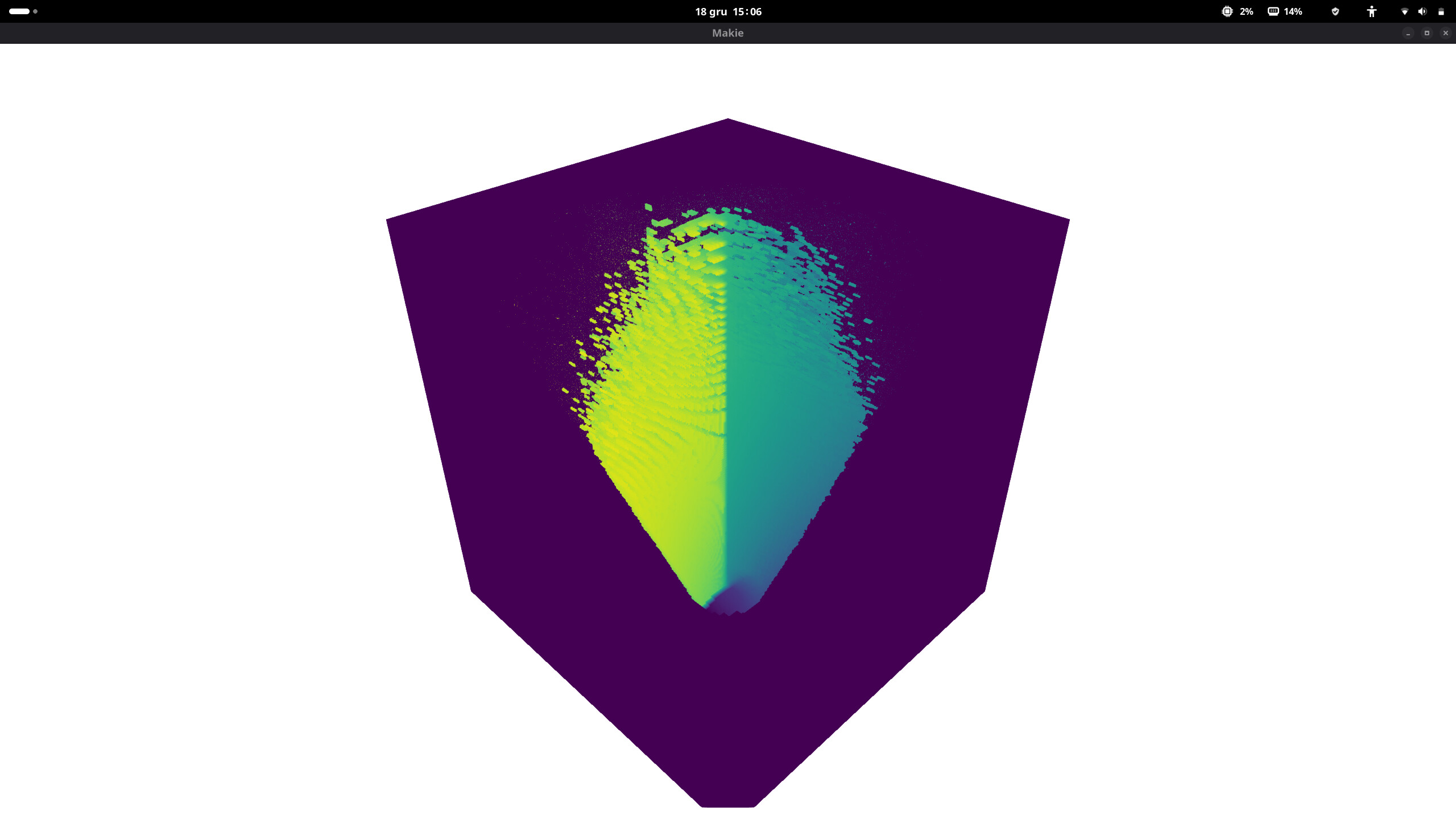
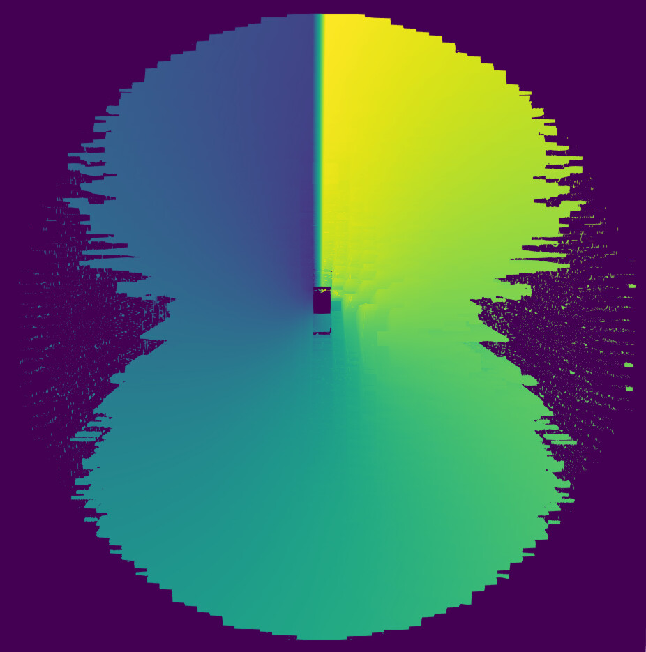
I am getting discrete/pixelated colors in 3D plot due to sampling in field variable in MWE code below. Why it is discretized and how to solve it?

using GLMakie
r = Float32[1.677044, 1.8385518, 2.0156136, 2.2097273, 2.4225352, 2.6558375, 2.911608, 3.1920104, 3.499417, 3.8364286, 4.205896, 4.6109447, 5.055002, 5.5418243, 6.0755296, 6.660634, 7.3020864, 8.005314];
θ = Float32[0.049087387, 0.14726216, 0.24543692, 0.3436117];
ϕ = Float32[0.19634955, 0.5890486, 0.9817477, 1.3744467, 1.7671459, 2.1598449, 2.552544, 2.9452431, 3.3379421, 3.7306414, 4.12334, 4.5160394, 4.9087386, 5.3014374, 5.6941366, 6.086836];
Bp_block = rand(18,4,16);

function cart(iex,ii,jj,kk,r_eval,θ_eval,ϕ_eval,X,Y,Z,C)
    rr, th, ph = r_eval[ii], θ_eval[jj], ϕ_eval[kk]
    xy, z = rr .* sincos(th)
    y, x = xy .* sincos(ph)
    X[iex] = x
    Y[iex] = y
    Z[iex] = z
    C[iex] = log(rr)+th+ph
end
function clp(X,Y,Z,C,xmin,ymin,zmin,sx,sy,sz,nx,ny,nz,field)	
	xi = trunc(Int, (X-xmin) * sx) + 1
	yi = trunc(Int, (Y-ymin) * sy) + 1
	zi = trunc(Int, (Z-zmin) * sz) + 1
	ix = clamp(xi, 1, nx)
	iy = clamp(yi, 1, ny)
	iz = clamp(zi, 1, nz)
	field[ix, iy, iz] = C
end

nx,ny,nz = 190, 50,170
xmin, xmax, ymin, ymax, zmin, zmax = -3.2042396f0, 3.2042396f0, -3.2042396f0, 3.2042396f0, 1.4782072f0, 8.373081f0;
sx::Float32 = (nx-1)/(xmax-xmin); sy::Float32 = (ny-1)/(ymax-ymin); sz::Float32 = (nz-1)/(zmax-zmin)
field = fill(NaN32, nx,ny,nz)
r_eval = exp.(LinRange(log(1.6), log(8.373081), nx))
θ_eval = LinRange(0.0, 0.3926991, ny)
ϕ_eval = LinRange(0.0, 6.2831855, nz)
X, Y, Z, C= ntuple(_ -> Vector{Float32}(undef, nx*ny*nz), 4);
global iex::Int32 = 1
@inbounds for ii in 1:nx, jj in 1:ny, kk in 1:nz
	cart(iex,ii,jj,kk,r_eval,θ_eval,ϕ_eval,X,Y,Z,C)
	clp(X[iex],Y[iex],Z[iex],C[iex],xmin,ymin,zmin,sx,sy,sz,nx,ny,nz,field)
	global iex += 1
end

function tdplot(xmin, xmax, ymin, ymax, zmin, zmax, field)
    fig = Figure()
    ax::LScene = LScene(fig[1,1], show_axis=false)
	volume!(ax, xmin..xmax, ymin..ymax, zmin..zmax, field)
	display(fig)
end
tdplot(xmin, xmax, ymin, ymax, zmin, zmax, field)

:down_arrow: Notice the discrete voxels in upper part.

If I understand your code correctly, you sample a function in spherical coordinates to fill in a field in cartesian coordinates (with a grid of (nx,ny,nz) ) , which you then plot. But then using nx,ny and nz in the sampling of the spherical coordinates as you do (nx along r, ny and nz along angles) does not make much sense and you probably never fill in the cartesian grid, even in the region where your spherical coordinates provide data, simply because the steps from the spherical grids might jump over the grid steps in cartesian coordinates. Here is what you get if you use another resolution nxs,nys,nzs (more points than nx,ny,nz) for the sampling in the spherical space than in the cartesian space

I don’t want to fill Cartesian grid completely because it will look like Cuboid but actually it is frustum or truncated cone in spherical coordinate.

I have tried it earlier but it starts looking like step well and is not smooth on increasing samples along x, y and z direction.

As far as I can see, the biggest problem here is how you sample the grid. If done this way, you have MUCH more points with low r than with high r — hence the artifacts in the upper part, where the r is high. To make it more uniform, you can do something like this:

# ...
r_eval = cbrt.(LinRange(1.6^3, 8.373081^3, nx))
θ_eval = acos.(LinRange(cos(0), cos(0.3926991), ny))
# ...

This is because the volume element in spherical coordinates is dV = r^2 \sin(\theta) dr d\theta d\phi.

Besides, what do you even want to visualize here? The value on the surface? Maybe the mesh plot will suit your needs better here?

2 Likes

Thanks, I want to get volume plot. I have earlier tried Meshes.jl but it is useless for my case as it does not have volume interpolation feature.

I still get discrete/pixelated plot even after inserting above code.


I am using endpoints of re(geometric series), θe(arithmetic) and ϕe(arithmetic series) in r_eval, θ_eval and ϕ_eval creation.

using Meshes, CoordRefSystems
re =  Float32[1.6, 1.754088, 1.9230156, 2.1082115, 2.311243, 2.5338273, 2.7778475, 3.0453684, 3.3386526, 3.6601818, 4.012676, 4.3991165, 4.8227735, 5.287231, 5.7964177, 6.354642, 6.9666257, 7.637547, 8.373081]
θe = Float32[0.0, 0.09817477, 0.19634955, 0.2945243, 0.3926991]
ϕe = Float32[0.0, 0.3926991, 0.7853982, 1.1780972, 1.5707964, 1.9634954, 2.3561945, 2.7488935, 3.1415927, 3.5342917, 3.9269907, 4.3196898, 4.712389, 5.105088, 5.497787, 5.8904862, 6.2831855]
g = RectilinearGrid{𝔼, typeof(Spherical(0,0,0))}((re, θe, ϕe))
viz(g)

I still do not know exactly what you want to achieve but as said in several replies, your sampling rate is not adapted to the final grid you want to plot. Just to show, I increased the resolution in the spherical space (and got rid of the X,Y,Z,C arrays which are actually never really used). Also note that with your approach, the value of field(i,j,k) might depend on the order in which you scan your spherical grid, since several points can land on discrete point (i,j,k) in cartesian coordinates and you keep the last value.
I will stop here.

using GLMakie
r = Float32[1.677044, 1.8385518, 2.0156136, 2.2097273, 2.4225352, 2.6558375, 2.911608, 3.1920104, 3.499417, 3.8364286, 4.205896, 4.6109447, 5.055002, 5.5418243, 6.0755296, 6.660634, 7.3020864, 8.005314];
θ = Float32[0.049087387, 0.14726216, 0.24543692, 0.3436117];
ϕ = Float32[0.19634955, 0.5890486, 0.9817477, 1.3744467, 1.7671459, 2.1598449, 2.552544, 2.9452431, 3.3379421, 3.7306414, 4.12334, 4.5160394, 4.9087386, 5.3014374, 5.6941366, 6.086836];
Bp_block = rand(18,4,16);

function cart(iex,ii,jj,kk,r_eval,θ_eval,ϕ_eval,X,Y,Z,C)
    rr, th, ph = r_eval[ii], θ_eval[jj], ϕ_eval[kk]
    xy, z = rr .* sincos(th)
    y, x = xy .* sincos(ph)
    X[iex] = x
    Y[iex] = y
    Z[iex] = z
    C[iex] = log(rr)+th+ph
end
function clp(X,Y,Z,C,xmin,ymin,zmin,sx,sy,sz,nx,ny,nz,field)	
	xi = trunc(Int, (X-xmin) * sx) + 1
	yi = trunc(Int, (Y-ymin) * sy) + 1
	zi = trunc(Int, (Z-zmin) * sz) + 1
	ix = clamp(xi, 1, nx)
	iy = clamp(yi, 1, ny)
	iz = clamp(zi, 1, nz)
	field[ix, iy, iz] = C
end

nx,ny,nz = 190, 50,170
nxs,nys,nzs=500,500,500
xmin, xmax, ymin, ymax, zmin, zmax = -3.2042396f0, 3.2042396f0, -3.2042396f0, 3.2042396f0, 1.4782072f0, 8.373081f0;
sx::Float32 = (nx-1)/(xmax-xmin); sy::Float32 = (ny-1)/(ymax-ymin); sz::Float32 = (nz-1)/(zmax-zmin)
field = fill(NaN32, nx,ny,nz)
r_eval = exp.(LinRange(log(1.6), log(8.373081), nxs))
θ_eval = LinRange(0.0, 0.3926991, nys)
ϕ_eval = LinRange(0.0, 6.2831855, nzs)
X, Y, Z, C= ntuple(_ -> Vector{Float32}(undef, 1),4);#nx*ny*nz), 4);
global iex::Int32 = 1
@inbounds for ii in 1:nxs, jj in 1:nys, kk in 1:nzs
	cart(iex,ii,jj,kk,r_eval,θ_eval,ϕ_eval,X,Y,Z,C)
	clp(X[iex],Y[iex],Z[iex],C[iex],xmin,ymin,zmin,sx,sy,sz,nx,ny,nz,field)
	#global iex += 1
end

function tdplot(xmin, xmax, ymin, ymax, zmin, zmax, field)
    fig = Figure()
    ax::LScene = LScene(fig[1,1], show_axis=false)
	volume!(ax, xmin..xmax, ymin..ymax, zmin..zmax, field)
	display(fig)
end
tdplot(xmin, xmax, ymin, ymax, zmin, zmax, field)

2 Likes

Thanks @JM_Beckers It improved quality of my 3D volume plot.

full code
using GLMakie, Interpolations
r = Float32[1.677044, 1.8385518, 2.0156136, 2.2097273, 2.4225352, 2.6558375, 2.911608, 3.1920104, 3.499417, 3.8364286, 4.205896, 4.6109447, 5.055002, 5.5418243, 6.0755296, 6.660634, 7.3020864, 8.005314];
θ = Float32[0.049087387, 0.14726216, 0.24543692, 0.3436117];
ϕ = Float32[0.19634955, 0.5890486, 0.9817477, 1.3744467, 1.7671459, 2.1598449, 2.552544, 2.9452431, 3.3379421, 3.7306414, 4.12334, 4.5160394, 4.9087386, 5.3014374, 5.6941366, 6.086836];
Bp_block = rand(18,4,16);

function cart(iex,ii,jj,kk,r_eval,θ_eval,ϕ_eval,ext_itp,X,Y,Z,C)
    rr, th, ph = r_eval[ii], θ_eval[jj], ϕ_eval[kk]
    xy, z = rr .* sincos(th)
    y, x = xy .* sincos(ph)
    X[iex] = x
    Y[iex] = y
    Z[iex] = z
    C[iex] = ext_itp(log(rr), th, ph)
end
function clp(X,Y,Z,C,xmin,ymin,zmin,sx,sy,sz,nx,ny,nz,field)	
	xi = trunc(Int, (X-xmin) * sx) + 1
	yi = trunc(Int, (Y-ymin) * sy) + 1
	zi = trunc(Int, (Z-zmin) * sz) + 1
	ix = clamp(xi, 1, nx)
	iy = clamp(yi, 1, ny)
	iz = clamp(zi, 1, nz)
	field[ix, iy, iz] = C
end

nx,ny,nz = 230, 50,190
nxs,nys,nzs = 2nx,2ny,3nz  	#500, 500,500
xmin, xmax, ymin, ymax, zmin, zmax = -3.2042396f0, 3.2042396f0, -3.2042396f0, 3.2042396f0, 1.4782072f0, 8.373081f0;
sx::Float32 = (nx-1)/(xmax-xmin); sy::Float32 = (ny-1)/(ymax-ymin); sz::Float32 = (nz-1)/(zmax-zmin)
field = fill(NaN32, nx,ny,nz)
ext_itp = extrapolate(interpolate((log.(r), θ, ϕ), Bp_block, Gridded(Linear())), Interpolations.Line())
r_eval = exp.(LinRange(log(1.6), log(8.373081), nxs))
#r_eval = cbrt.(LinRange(1.6^3, 8.373081^3, nxs))
θ_eval = acos.(LinRange(cos(0), cos(0.3926991), nys))
ϕ_eval = LinRange(0.0, 6.2831855, nzs)
X, Y, Z, C= ntuple(_ -> Vector{Float32}(undef, 1), 4);
global iex::Int32 = 1
@inbounds for ii in 1:nxs, jj in 1:nys, kk in 1:nzs
	cart(iex,ii,jj,kk,r_eval,θ_eval,ϕ_eval,ext_itp,X,Y,Z,C)
	clp(X[iex],Y[iex],Z[iex],C[iex],xmin,ymin,zmin,sx,sy,sz,nx,ny,nz,field)
end

function tdplot(xmin, xmax, ymin, ymax, zmin, zmax, field)
    fig = Figure()
    ax::LScene = LScene(fig[1,1], show_axis=false)
	volume!(ax, xmin..xmax, ymin..ymax, zmin..zmax, field)
	display(fig)
end
tdplot(xmin, xmax, ymin, ymax, zmin, zmax, field)

Do you still doubt correctness of my method?