Control systems, pid, and high-order transfer functions

Hello,

It’s specific to control systems and this is my first post, so I still decided to post under “new to Julia” as I might be asking beginner questions.

I’m making a 1-dimension model of the PX4 cascaded control loops. PX4 is a controller for drones.

There are 4 cascaded loops. Let’s call then Gx (position closed loop), Gv (vel CL), Gout (angle CL), and Gin (rate CL). The closed loops obviously include the plant (i.e. the 1D model for the drone).

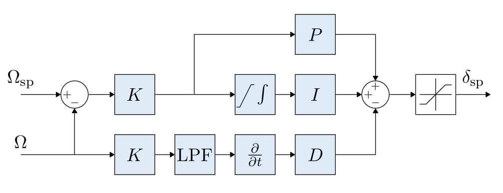
The rate loop is a PID, however as you can see, the D-term does not multiply the reference AND its signal is low pass filtered. We’ll omit the saturation as this is non-linear.

I derived the equations by hand and I obtained Gin (although it looks like ControlSystemsBase.pid_2dof() could have done exactly that)

TransferFunction{Continuous, ControlSystemsBase.SisoRational{Float64}}
                    1.7664s^3 + 8.8576s^2 + 5.120000000000001s
----------------------------------------------------------------------------------
0.00046575s^6 + 0.022725s^5 + 0.32s^4 + 2.8432s^3 + 8.8576s^2 + 5.120000000000001s

First question: how can I simplify this transfer function? I would like to divide the num and denominator by s.

I’m able to obtain the polynomial with Gin.matrix[1].num and Gin.matrix[1].den, then impossible to divide them.
Here is a code snippet so you can help me solve it

# transfer functions example in Julia - July 18, 2025 - Romain Chiappinelli
using Plots
using ControlSystemsBase, LinearAlgebra, ControlSystems
using RobustAndOptimalControl
plotly();

Gin=tf([1.7664, 8.8576, 5.120000000000001, 0],[0.00046575, 0.022725, 0.32, 2.8432, 8.8576, 5.120000000000001, 0])
if Gin.matrix[1].num(0)==0 && Gin.matrix[1].den(0)==0
   # what to do here ?
end

Then I close the loop with the P term. I obtain a 14 order polynomial at the denominator, which could be reduced to order 11 by answering question 1.

s=tf("s")
P=2.5
Gout = (P*Gin) / (s+P*Gin)

and I obtain the following warning.

Warning: High-order transfer functions are highly sensitive to numerical errors. The result may be inaccurate. Consider making use of statespace systems instead

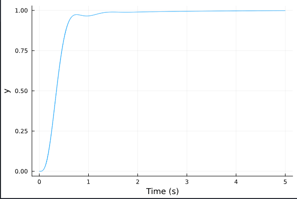
At this point, I’m still able to do a step response that matches the real data. Spoiler alert: late on, Gv will have order 22 and the step response does not match the reality :grinning_face_with_smiling_eyes:
Then, when I do

Gins=ss(Gin)
Gout = ss((P*Gins) / (s+P*Gins))

it tells me System is improper, a state-space representation is impossible. Any mathematical explanation cue?
Testing the code as I write this topic, I realized that this works

Gins=ss(Gin)
Gout = ss((P*Gins/s) / (1+P*Gins/s))

I think the topic is half resolved now. and by closing the loops properly I’ll be able to to have a proper system and have my step response.

Do you think the order 22 as a state space will give me accurate results?

1 Like

maybe:

julia> sys = tf([1.7664, 8.8576, 5.120000000000001, 0], [0.00046575, 0.022725, 0.32, 2.8432, 8.8576, 5.120000000000001, 0])
TransferFunction{Continuous, ControlSystemsBase.SisoRational{Float64}}
                    1.7664s^3 + 8.8576s^2 + 5.120000000000001s
----------------------------------------------------------------------------------
0.00046575s^6 + 0.022725s^5 + 0.32s^4 + 2.8432s^3 + 8.8576s^2 + 5.120000000000001s

Continuous-time transfer function model

julia> minreal(sys)
TransferFunction{Continuous, ControlSystemsBase.SisoRational{Float64}}
                            3792.592592592592s^2 + 19017.928073000534s + 10993.02200751476
----------------------------------------------------------------------------------------------------------------------
1.0s^5 + 48.79227053140099s^4 + 687.0638754696727s^3 + 6104.562533548038s^2 + 19017.928073000523s + 10993.022007514752

Continuous-time transfer function model

edit: forgot to say, first welcome to this community :laughing::raised_hand:

2 Likes

minreal(Gin) simplifies the transfer function.

Don’t do this, use the function feedback(P*Gin) = P*Gin/(1+P*Gin) instead. Is the s in the denominator deliberate or a typo?

Yes, it’s generally better to convert your systems to statespace representation using the function ss. Do this is soon as possible. See Performance considerations · ControlSystems.jl for some details as to why.

likely due to the non-minimal realization.

Try

Gin=tf([1.7664, 8.8576, 5.120000000000001, 0],[0.00046575, 0.022725, 0.32, 2.8432, 8.8576, 5.120000000000001, 0])
Gin = ss(Gin)
Ginr = minreal(Gin, 1e-8)
Gout = feedback(P*Gin)
2 Likes

Statespace simulation can be accurate up to any arbitrarily high order provided that the realization is properly balanced, which it’ll be by default upon conversion from a transfer function.

If you use mineral and feedback as suggested above, you should get a much smaller order of the final system though.

1 Like

Amazing for those quick replies!
yeah minreal() that simple :slight_smile:

Yes, the s in the denominator is deliberate. The plant seen by the outer loop is in fact Gin/s.

I’ll give it a try to the full loop and come back to you.

In that case I think forming Gin/s and then calling feedback is the best approach. You can also divide Gin by s already at construction by just removing the last zero in the numerator coefficient array.

using ControlSystemsBase, Plots
Gins = tf(
    [1.7664, 8.8576, 5.120000000000001],
    [0.00046575, 0.022725, 0.32, 2.8432, 8.8576, 5.120000000000001, 0]
) |> ss
P=2.5

Gout = feedback(P*Gins)
plot(step(Gout, 5))

This results in a low-order system

julia> Gout = feedback(P*Gins)
StateSpace{Continuous, Float64}
A = 
 -48.79227053140096  -21.470746108427267  -11.922973698336017  -6.957863660762211  -7.14573268921095  -3.3548040794417613
  32.0                 0.0                  0.0                 0.0                 0.0                0.0
   0.0                16.0                  0.0                 0.0                 0.0                0.0
   0.0                 0.0                  8.0                 0.0                 0.0                0.0
   0.0                 0.0                  0.0                 2.0                 0.0                0.0
   0.0                 0.0                  0.0                 0.0                 1.0                0.0
B = 
 2.0
 0.0
 0.0
 0.0
 0.0
 0.0
C = 
 0.0  0.0  0.0  1.1574074074074072  2.9019055287171227  1.6774020397208806
D = 
 0.0

Continuous-time state-space model

Hello,

Thanks a lot for all the support!

I was able to implement all the loops. The position loop has order 12 (outer most loop), and everything is working nice and quick.

I created my feedback loops from the doc of pid_2dof. Since it allows only a first order low pass filter, I created my own Cr and Cy

s=tf("s")
IMU_DGYRO_CUTOFF=30
wd=IMU_DGYRO_CUTOFF*2*pi	# Hz to rad/s
faa=wd^2/(s+wd)^2
k=1; kp=k*0.2; ki=k*0.2; kd=k*0.003; kf=k*0.0;

P_drone=ss(tf([7901.2],[1, 44.44, 493.827, 0]))
Cr=ss(kp+ki/s+kf)
Cy=ss(minreal(kp+ki/s+kd*s*faa))
Gin=minreal(feedback(P_drone, Cy)*Cr)

101 question: I have to express my filters into rad/s to obtain the correct step response, right?

In that case I think forming Gin/s and then calling feedback is the best approach.

Yes, I used this approach.

And thanks for the link to the performance considerations, it lists subtleties that are well explained and shown through examples.

1 Like

Yes, any frequencies like your wd above would be expressed in rad/s, so wd=IMU_DGYRO_CUTOFF*2*pi looks correct.