Computational performance when broadcasting a convolution layer

For 2D images, the usual input format for Conv layers is Array{Float32, 4}. I’m currently experimenting with broadcasting a Conv layer over a Vector{Array{Float32, 4}}, however I have found the performance to be significantly worsened by this approach.

using Flux
using BenchmarkTools

const w = 16   # image width
const h = 16   # image height
CNN = Conv((5, 5), 1 => 4) # arbitrarily chosen architecture

X = rand(Float32, w, h, 1, 1000)
@btime CNN($X)
# 1.606 ms (58 allocations: 4.45 MiB)

X = [rand(Float32, w, h, 1, 1) for _ ∈ 1:1000]
@btime CNN.($X)
# 14.195 ms (56000 allocations: 62.69 MiB)

This performance discrepancy increases as the architecture complexity increases. Does anyone know why there is a performance discrepancy? (There are reasons why I would want to use this structure.)

The difference in allocations probably accounts for most of the discrepancy. In the broadcast case, all the intermediates needed must be re-allocated for each application of the model. In the other case, you get a few big allocations. In addition, it is often the case on modern systems (especially when you use a GPU, but even on CPUs) that one big matrix multiply is faster than many small matrix multiplies.

One possible solution is to use RecursiveArrayTools.jl which would allow you to view the data as a vector of arrays or as one big array as needed.

1 Like

I assume in practice you would be using minibatches instead of batches of size 1, so the effect should be less pronounced. It might not hurt to articulate why this is desired though, as other than memory liminations I can’t think of any reason to use a smaller batch size.

Thanks very much for the comments.

As TouchSir notes, some context may be helpful (I wanted to keep the MWE as simple as possible, but that simplicity has probably been a hindrence).

At m locations, we have n_i, i = 1, \dots, m, univariate (single channel) 16 \times 16 input images. In the original example, we have a single image at each location, so n_i = 1: However, in practice, n_i can be any positive integer and is not necessarily constant. For each location, I need to apply a CNN to each of the n_i images, and then aggregate the resulting n_i outputs associated with a given location.

Some code which should add clarity. If we have m = 1000 locations and between 20 and 40 images at each location, then I would do the following (including an attempt at using RecursiveArrayTools.jl, as per contradict’s suggestion):

using RecursiveArrayTools

m = 1000
n = rand(20:40, m)
X = [rand(Float32, w, h, 1, n[i]) for i ∈ eachindex(n)]

@btime CNN.($X)
# 177.813 ms (58225 allocations: 190.71 MiB)

A = ArrayPartition(X...)
@btime CNN.($A.x)
# 169.872 ms (58003 allocations: 190.14 MiB)

X = VectorOfArray(X)
@btime CNN.($X.u) 
# 172.439 ms (58103 allocations: 190.13 MiB)

(I may not have implemented RecursiveArrayTools.jl as contradict had intended; please let me know if this is the case.) For comparison with a similar amount of data using the traditional approach of feeding in a single large array:

X = rand(Float32, w, h, 1, 30 * 1000)
@btime CNN($X)
# 73.520 ms (58 allocations: 131.89 MiB)

I think this supports contradict’s point, that the poor performance comes from using many small arrays rather than one large array. Perhaps there is a better approach than broadcasting over a vector of arrays? I have looked into DepthwiseConv layers, but I don’t think it’s exactly what I need, and it doesn’t seem to work on the GPU.

Thanks for the explanation. AIUI, you just need to be able to aggregate the CNN outputs for each location? If so, then it should be sufficient to run the model over the entire batch and then do the aggregation. This assumes there are no layers like batchnorm present which break the independence of samples in the batch. It’s not the end of the world if you do have those layers either, but there will likely be more work involved (less so if you’re only concerned about inference).

Hi, sorry for the delayed response.

Yes, that’s right. Appreciate the suggestion, and I spent some time exploring it. I did some tests on the run-time and memory performance using the “Array” method, which applies the CNN to one large array of images, and the “VecArray” method, which broadcasts the CNN over a vector of arrays of images. I was interested to see how performance changes with

  • the size of the CNN, in terms of the number of trainable parameters,
  • m, the number of “locations”; that is, the number of elements in the vector that we are broadcasting over, and
  • n_i, the number of images at each location; that is, the number of images stored in each element of the vector.

I looked at two CNNs, one with ~100 parameters, and another with ~420,000 parameters. The large CNN is reflective of the size of network I am using in my application. I used all combinations of m \in \{16, 32, 64, 128\} and n _i \in \{1, 10, 25, 50, 75, 100\}. (These values of m are reflective of typical mini-batch sizes.)

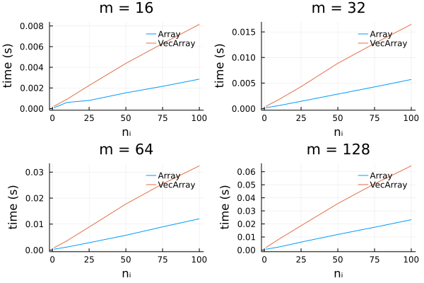
Run-times: Using the small CNN yields a large discrepancy between run-times, while there is little difference when using the large CNN:

Small CNN (~100 parameters):

CNN1_time

Large CNN (~420,000 parameters):

CNN2_time

Memory usage: there appears to be a constant penalty to using the Vector{Array} approach, which is fixed for a given value of m (i.e., it does not change with n_i):

Small CNN (~100 parameters):

CNN2_memory

Large CNN (~420,000 parameters):

CNN1_memory

Note that this was done on the CPU: The results may change on the GPU. The results suggest that, for the large CNN, there isn’t a massive difference in terms of run time and memory usage when n_i is “large enough” (e.g., for n_i = 50).

I should note that I made a mistake by looking at the case of m = 1000 and n_i = 1 in my original question. In this configuration, applying a CNN to an array and then aggregating is indeed much better than broadcasting over a vector of arrays, but this is not practically relevant for my application.

Thanks again for your helpful comments!

3 Likes