Something seems strange indeed. I’m not an expert on ModelingToolkit.jl or BoundaryValueDiffEq.jl, but I can reproduce your issue on my machine.
versioninfo()
Julia Version 1.12.1
Commit ba1e628ee49 (2025-10-17 13:02 UTC)
Build Info:
  Official https://julialang.org release
Platform Info:
  OS: Linux (x86_64-linux-gnu)
  CPU: 64 × AMD Ryzen Threadripper PRO 3975WX 32-Cores
  WORD_SIZE: 64
  LLVM: libLLVM-18.1.7 (ORCJIT, znver2)
  GC: Built with stock GC
Threads: 1 default, 1 interactive, 1 GC (on 64 virtual cores)
Environment:
  JULIA_PKG_USE_CLI_GIT = true
  JULIA_MAX_NUM_PRECOMPILE_FILES = 50
Packages
  [764a87c0] BoundaryValueDiffEq v5.18.0
  [f3b72e0c] DiffEqDevTools v2.48.0
  [20393b10] InfiniteOpt v0.5.9
  [b6b21f68] Ipopt v1.12.1
  [961ee093] ModelingToolkit v10.26.1
  [91a5bcdd] Plots v1.41.1
BVProblem
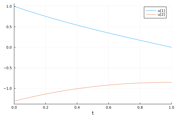
This version only using BoundaryValueDiffEq.jl (which I think matches your original set of equations?) seems to work fine and identifies the initial condition for dy ≈ -1.31.
using BoundaryValueDiffEq

function testproblem!(du, u, p, t)
    du[1] = u[2]
    du[2] = u[1]
end

function bc!(residual, u, p, t)
    residual[1] = u(ti)[1] - 1
    residual[2] = u(tf)[1]
end

prob = BVProblem(testproblem!, bc!, [1.0, 1.0], (ti, tf))
sol = solve(prob, MIRK4(), dt = 0.001)

Plots.plot(sol)
JuMPDynamicOptProblem
The code you tried with the Jump problem runs, but does the wrong thing:
using ModelingToolkit
using ModelingToolkit: t_nounits as t, D_nounits as D

@variables y(..)
eqs = [D(D(y(t))) ~ y(t)]

@parameters deriv_guess

(ti, tf) = (0.0, 1.0)
cons = [y(tf) ~ 0.0]

@named bvpsys = System(eqs, t; constraints=cons)
bvpsys = mtkcompile(bvpsys)

u0map = [y(t) => 1.0, D(y(t)) => deriv_guess]
parammap = [deriv_guess => -1.0]

using InfiniteOpt, Ipopt, DiffEqDevTools
jprob = JuMPDynamicOptProblem(bvpsys, [u0map; parammap], (ti, tf); dt=0.001)
jsol = solve(jprob, JuMPCollocation(Ipopt.Optimizer, constructRadauIIA5()))
As you mentioned the corresponding solution is clearly incorrect:
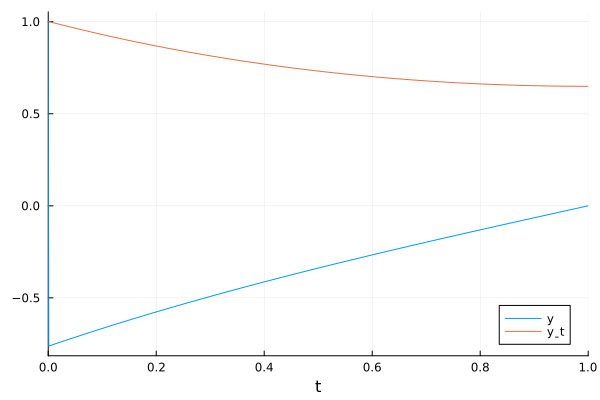
But I did get this warning which seems highly relevant:
┌ Warning: The control problem is overdetermined. The total number of conditions (# constraints + # fixed initial values given by op) exceeds the total number of states. The solvers will default to doing a nonlinear least-squares optimization.
└ @ ModelingToolkit ~/.julia/packages/ModelingToolkit/b28X4/src/systems/optimal_control_interface.jl:99
So (as the plot also suggests) the solution is actually just a least squares fit with three datapoints (y(ti), y(tf), and the specified initial dy(ti) which was not treated as guess but rather as a fixed initial condition. Since there is no solution of the equation that satisfies these three points, y(t) immediately jumps to what would be the correct initial condition for the other two points.
It reminds me of a recent thread here about this warning about overdetermined systems:
It’s a different problem type, but the solution there was to specify the initial condition to be determined as nothing. I tried that here, but it didn’t work:
u0map = [y(t) => 1.0, D(y(t)) => nothing]
parammap = []
jprob = JuMPDynamicOptProblem(bvpsys, [u0map; parammap], (ti, tf); dt=0.001)
ERROR: Initial condition underdefined. Some are missing from the variable map.
Please provide a default (`u0`), initialization equation, or guess
for the following variables:

yˍt(t)
… but specifying the “initial guess” leads to the above warning.
MTK into BVProblem
Your original approach actually “works” for me sometimes, in the sense that I could create the problem once, but also crashes with a segfault either at the solve step or the construction of the BVProblem. I couldn’t really find out more so far …
prob = BVProblem(bvpsys, [1.0, 1.0], (ti, tf))
sol = solve(prob, MIRK4(), dt=0.001)
Overall I feel like this should work. Perhaps there is really something wrong with how the conversion should happen (then the documentation should probably be improved). Or it’s a bug somewhere ![]()