Is it currently possible to symbolically setup and then numerically solve boundary-value problems using ModelingToolkit? This issue tells me this is possible through the dynamic optimization interface but I’m not sure how to set it up this way. As a test case I’m trying this simple example from the BoundaryValueDiffEq docs:
using BoundaryValueDiffEq
function f!(du, u, p, t)
    du[1] = u[2]
    du[2] = u[1]
end
function bc!(res, u, p, t)
    res[1] = u(0.0)[1] - 1
    res[2] = u(1.0)[1]
end
tspan = (0.0, 1.0)
u0 = [0.0, 0.0]
prob = BVProblem(f!, bc!, u0, tspan)
sol = solve(prob, MIRK4(), dt = 0.01)
Here is my attempt at setting this up in ModelingToolkit:
using ModelingToolkit
using ModelingToolkit: t_nounits as t, D_nounits as D
using BoundaryValueDiffEq # for BVProblem
@variables y(..)

eqs = [D(D(y(t))) ~ y(t)]

(ti, tf) = (0.0, 1.0)
cons = [y(ti) ~ 1.0, y(tf) ~ 0.0]

@named bvpsys = System(eqs, t; constraints=cons)
bvpsys = mtkcompile(bvpsys)

u0 = [0.0, 0.0]
prob = BVProblem(bvpsys, u0, (ti, tf))
# or do I need JuMPDynamicOptProblem() ?
sol = solve(prob, MIRK4(), dt=0.01)
My attempt above leads to a seg fault and my REPL crashes so something is horribly wrong. I’m guessing BVProblem is not the one to use here and I need a dynamic optimization solver like in these examples, but I’m not sure how. What is the proper syntax for this?
Did you end up trying it with JuMPDynamicOptProblem ?
From the docs page you linked it sounds like that is the recommended way to go and also shows how to use the problem. It should look roughly like this I guess.
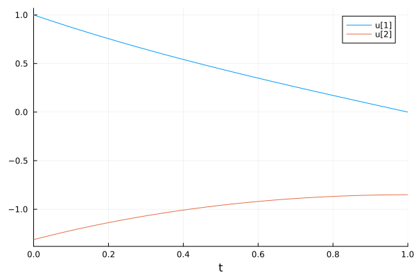
Thanks for the recommendation. I tried it this way by supplying a guess for the value of the derivative. However, the solution seems to rapidly course-correct after the initial timestep in order to satisfy the boundary conditions. This does not match the correct solution found with BoundaryValueDiffEq.jl. Not sure what I’m doing wrong.
I see here that the docs have BVProblem defined for the System type, so maybe there is a way to set up the problem without using dynamic optimization? If there is, I’d happily contribute documentation. It would be great to leverage the abilities of ModelingToolkit for these types of problems.
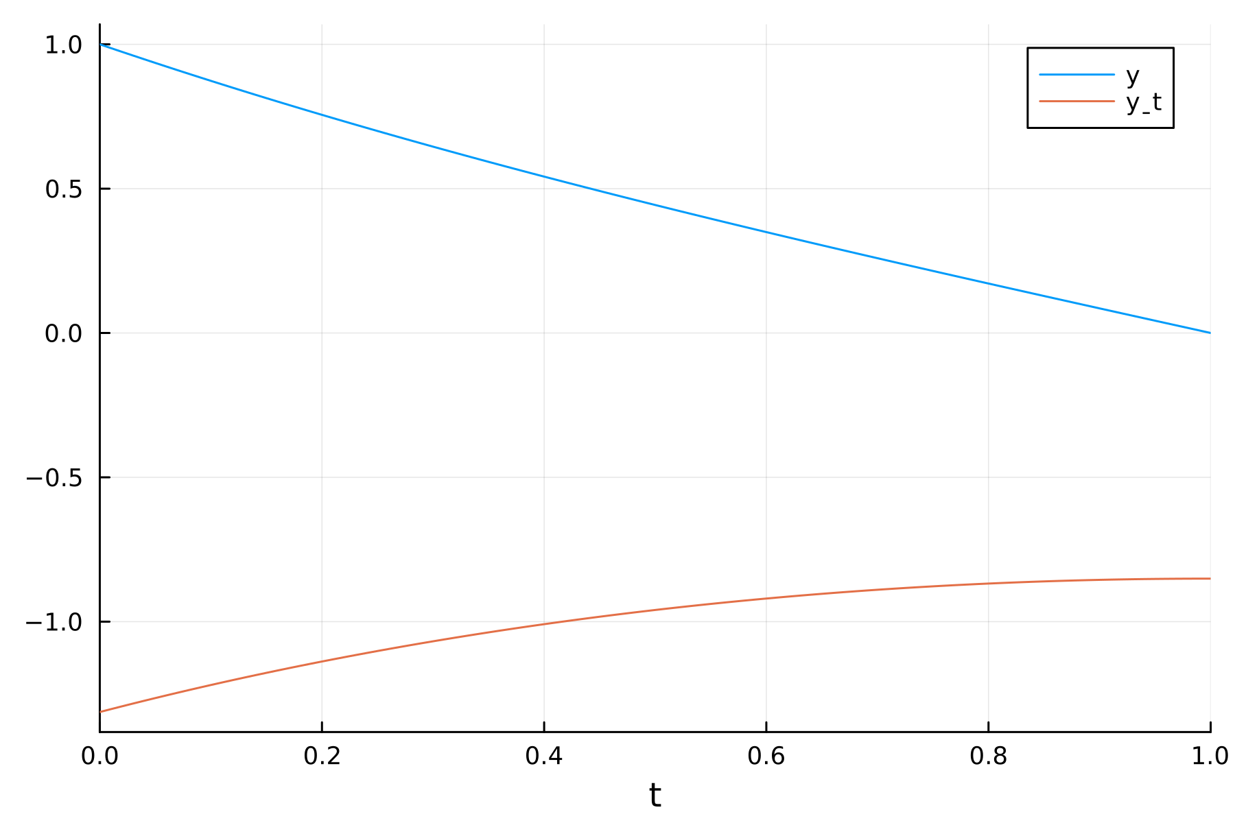
This version only using BoundaryValueDiffEq.jl (which I think matches your original set of equations?) seems to work fine and identifies the initial condition for dy ≈ -1.31.
using BoundaryValueDiffEq

function testproblem!(du, u, p, t)
    du[1] = u[2]
    du[2] = u[1]
end

function bc!(residual, u, p, t)
    residual[1] = u(ti)[1] - 1
    residual[2] = u(tf)[1]
end

prob = BVProblem(testproblem!, bc!, [1.0, 1.0], (ti, tf))
sol = solve(prob, MIRK4(), dt = 0.001)

Plots.plot(sol)
But I did get this warning which seems highly relevant:
┌ Warning: The control problem is overdetermined. The total number of conditions (# constraints + # fixed initial values given by op) exceeds the total number of states. The solvers will default to doing a nonlinear least-squares optimization.
└ @ ModelingToolkit ~/.julia/packages/ModelingToolkit/b28X4/src/systems/optimal_control_interface.jl:99
So (as the plot also suggests) the solution is actually just a least squares fit with three datapoints (y(ti), y(tf), and the specified initial dy(ti) which was not treated as guess but rather as a fixed initial condition. Since there is no solution of the equation that satisfies these three points, y(t) immediately jumps to what would be the correct initial condition for the other two points.
It reminds me of a recent thread here about this warning about overdetermined systems:
It’s a different problem type, but the solution there was to specify the initial condition to be determined as nothing. I tried that here, but it didn’t work:
ERROR: Initial condition underdefined. Some are missing from the variable map.
Please provide a default (`u0`), initialization equation, or guess
for the following variables:

yˍt(t)
… but specifying the “initial guess” leads to the above warning.
MTK into BVProblem
Your original approach actually “works” for me sometimes, in the sense that I could create the problem once, but also crashes with a segfault either at the solve step or the construction of the BVProblem. I couldn’t really find out more so far …
Overall I feel like this should work. Perhaps there is really something wrong with how the conversion should happen (then the documentation should probably be improved). Or it’s a bug somewhere
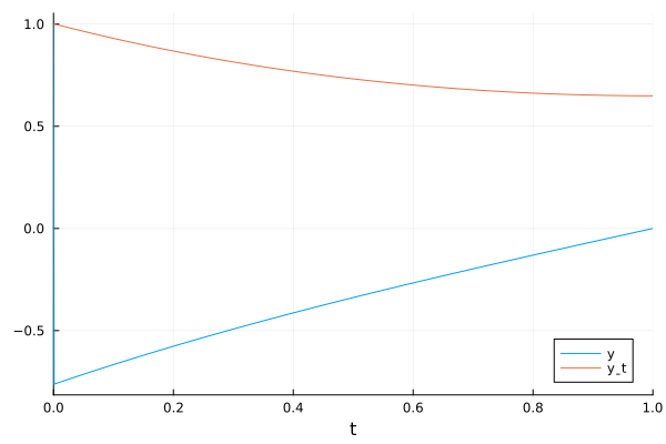
Okay, I think I got it now. My main issue was with how initial values were being passed to the solver. ModelingToolkit requires a vector of Pair objects mapping unknowns to their initial values. Guesses for unknown initial conditions or parameters are supplied via the guesses keyword argument. The following code produces the correct solution now!
using ModelingToolkit, BoundaryValueDiffEq, Plots
using ModelingToolkit: t_nounits as t, D_nounits as D

@variables y(..)
eq = [D(D(y(t))) ~ y(t)]

# right boundary condition treated as constraint
constr = [y(1.0) ~ 0.0]

@named bvp = System(
    eq, t;
    constraints=constr
)

bvpsys = mtkcompile(bvp)

# pass uncertain parameters/initial conditions to solver via `guesses`
prob = BVProblem(bvpsys, [y(t) => 1], (0.0, 1.0), guesses=[D(y(t)) => 0.0])
sol = solve(prob, MIRK4(), dt=0.01)
plot(sol)