[ANN] LoopVectorization

I’m excited to announce LoopVectorization.

LoopVectorization provides the @avx macro.
This macro can be prepended to a for loop or a broadcast statement, and it tries its best to vectorize the loop.
It can handle nested loops. It models the cost of evaluating the loop, and then unrolls either one or two loops.

Examples

Lets jump straight into the deep end with the classic: matmul.

@inline function gemmavx!(C, A, B)
    @avx for i ∈ 1:size(A,1), j ∈ 1:size(B,2)
        Cᵢⱼ = 0.0
        for k ∈ 1:size(A,2)
            Cᵢⱼ += A[i,k] * B[k,j]
        end
        C[i,j] = Cᵢⱼ
    end
end

For comparison, we have:

  1. Intel MKL, single threaded.
  2. Julia (@inbounds and @simd)
  3. Clang + Polly
  4. GFortran
  5. GFortran, matmul intrinsic
  6. icc
  7. ifort
  8. ifort, matmul intrinsic

You can see the Julia code I used to run the benchmarks here. The C and Fortran code are in the “looptest.c” and “looptest.f90” files of the same directory. The “driver.jl” file contains the script I ran to run the benchmarks (note, as is, it will run benchmarks in parallel; take care that this doesn’t cause problems).
loadsharedlibs.jl contains the commands (and flags) I used to compile the C and Fortran code.

I’ll add the new Flang once it is released. It is an LLVM Fortran compiler that uses MLIR, making it promising.

I benchmarked A * B, A' * B, and A * B'.
To represent LoopVectorization.jl, I used the gemmavx! function above for all three.
Each of the others, however, required a new function for each version.

A * B

I used the following Julia function (and the same order for C and Fortran):

function jgemm!(C, A, B)
    C .= 0
    M, N = size(C); K = size(B,1)
    @inbounds for n ∈ 1:N, k ∈ 1:K
        @simd ivdep for m ∈ 1:M
            C[m,n] += A[m,k] * B[k,n]
        end
    end
end

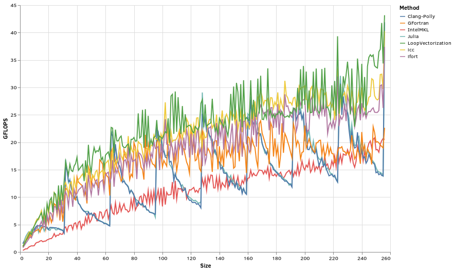
The plots cover all square matrices of sizes 2x2 through 256x256.
MKL is of course the fastest. Its performance drops once it starts running out of L2 cache.
LoopVectorization does second best. Its performance peaks between 40x40 and 64x64 matrices, but the performance is fairly steady over the size range after that.

Of the others, gfortran’s matmul intrinsic performs best as a function of matrix size, steadily increasing in performance, starting to take 3rd place at around 140x140.
Both Intel-Fortran versions were just on it’s heals over that range, and well ahead for matrices smaller than 140x140.

Throughout these benchmarks, Clang-Polly and Julia’s performance are highly variable, a “signature” of LLVM’s loop optimizer. But it did better than icc, gfortran-loops, and Julia.

A’ * B

Now we have A' * B:

@inline function jgemm!(C, Aᵀ::Adjoint, B)
    A = parent(Aᵀ)
    @inbounds for n ∈ 1:size(C,2), m ∈ 1:size(C,1)
        Cₘₙ = zero(eltype(C))
        @simd ivdep for k ∈ 1:size(A,1)
            Cₘₙ += A[k,m] * B[k,n]
        end
        C[m,n] = Cₘₙ
    end
end

Note that every function receiving transposed (adjoint) matrices was made @inline to avoid the allocation of tranposing the array. Perhaps I will just preallocate the tranpose the next time I update the benchmarks.
Here, we are essentially taking M * N dot products (where C is an M by N matrix), as we iterate over the M columns of A and N columns of B. As discussed later alongside the dot product benchmarks, the limiting factor is the rate at which the CPU can perform loads. Blocking – that is, loading from 4 columns of A and 4 columns of B to perform 4*4=16 products – helps us achieve much higher GFLOPS here than with the single dot products.

I don’t know what MKL is doing here, but it attains nearly the same performance as when A is not tranposed, which is not something I’ve been able to manage. Perhaps it somehow packs very efficiently to transpose A?

LoopVectorization and the three Intel-compiled functions are all probably doing the same thing: evaluating the loop order as written for the naive version, but blocked somehow to get a lot more arithmetic done per load.

GFortran (loops or built in), Clang-Polly, and Julia do not, and are therefore slow.

A * B’

This one is a lot like A * B, in that the most efficient algorithm involves loading contiguous elements from A and broadcasting scalars from B. B is just traversed in a different order.


Yet that change was enough to throw off implementations that get by more based on pattern matching vs an actual vectorization model, namely gfortran’s matmul intrinsic – you’d naturally expect a matmul function to be specially optimized, and it’s merely unfortunate that they don’t seem to have fast versions for the transpose – or Polly, which tries to detect matmul and emit fast code.

MKL is obviously fastest. LoopVectorization is next, followed by all three intel-compiled versions.

Dot Products

To get into a little about how it works, lets start with a simple example, a dot product:

function jdot(a, b)
    s = 0.0
    @inbounds @simd ivdep for i ∈ eachindex(a, b)
        s += a[i] * b[i]
    end
    s
end
function jdotavx(a, b)
    s = 0.0
    @avx for i ∈ eachindex(a, b)
        s += a[i] * b[i]
    end
    s
end

Most recent CPUs are capable of 2x aligned loads, and 2x fma per clock cycle.
Because the dot product requires 2 loads per fma, that bottle necks us at 1 fma per clock cycle.
However, it takes 4 clock cycles to complete an fma instruction on many recent CPUs. And to complete one iteration of s_new = s_old a[i] * b[i], we need to have calculated s_old.
For this reason, LoopVectorization unrolls the loop by a factor of 4, so that we have four copies of s, and a new fma instruction can be started on every clock cycle.

The worst performer here is Julia’s builtin dot (which I believe uses BLAS), which isn’t too surprisng here.
Next worst are the two LLVM-loop-optimized versions, suffering from highly variable performance based on the length of the loop remainders. At their peak, they match the competition, but Julia and Clang-Polly quickly fall off to the bottom from there.
gfortran isn’t doing too well either. I’d have to look more into what is going on there.

Now, consider the selfdot:

function jselfdot(a)
    s = 0.0
    @inbounds @simd ivdep for i ∈ eachindex(a)
        s += a[i] * a[i]
    end
    s
end
function jselfdotavx(a)
    s = 0.0
    @avx for i ∈ eachindex(a)
        s += a[i] * a[i]
    end
    s
end

Here we only need a single load per fma, meaning that it could potentially perform 2 fmas per clock cycle, requiring 8 concurrent instances.
But LLVM still unrolls it by a factor of 4.


However, that doesn’t seem to limit its peak performance. Perhaps because none of the functions are achieving half the GFLOPS of matrix multiplication: the fma units are spending at least half their time idle.
The pattern is similar to what we saw for the single argument dot product.

Three-argument, generalized, dot product

This computes x * A * y.

function jdot3(x, A, y)
    M, N = size(A)
    s = zero(promote_type(eltype(x), eltype(A), eltype(y)))
    @inbounds for n ∈ 1:N
        @simd ivdep for m ∈ 1:M
            s += x[m] * A[m,n] * y[n]
        end
    end
    s
end
function jdot3avx(x, A, y)
    M, N = size(A)
    s = zero(promote_type(eltype(x), eltype(A), eltype(y)))
    @avx for m ∈ 1:M, n ∈ 1:N
        s += x[m] * A[m,n] * y[n]
    end
    s
end

Like in A' * B, we can improve performance a lot by blocking. A single load from x can be multiplied with several loads of y, and vice versa. Recognizing this is a boon for performance:

When operating on matrices (and forced to do vector loads instead of broadcasts), LoopVectorization does best when the number of rows in the matrix is a multiple of 8. This is because when this happens, each of its columns will be 64 byte alligned, and the CPU can load 2 vectors per clock cycle. Othererwise, it can only load once per clock cycle from each column whose start isn’t at a memory address divisble by 64.
The effect is particularly striking here, because we do not get any reuse out of a load from A; we need 1 load from A per [multiplication & fma], meaning it must constantly be loading.

LoopVectorization does best here, while icc and ifort are close behind.
MKL here meant using the 3-argument dot(x, A, y), new to Julia 1.4.
I haven’t looked into how it’s implemented, but am guessing it is pure Julia based on how the performance behaves as a function of input size: like the other two LLVM versions.

Matrix * vector

‘gemv’ benchmarks, A * x:

function jgemv!(y, A, x)
    y .= 0.0
    @inbounds for j ∈ eachindex(x)
        @simd ivdep for i ∈ eachindex(y)
            y[i] += A[i,j] * x[j]
        end
    end
end
@inline function jgemvavx!(y, A, x)
    @avx for i ∈ eachindex(y)
        yᵢ = 0.0
        for j ∈ eachindex(x)
            yᵢ += A[i,j] * x[j]
        end
        y[i] = yᵢ
    end
end


I went into detail into matrix-vector multiplication here.
I think LoopVectorization did best over this range, but by the end MKL and gfortran began to overtake it.
LoopVectorization does not model memory yet. Ideally it would perform some blocking pattern that has better memory access patterns, but this is what we get for now,

We also consider A' * x, which is equivalent to x' * A (row-vector * matrix multiplciation):

@inline function jgemv!(y, Aᵀ::Adjoint, x)
    A = parent(Aᵀ)
    @inbounds for i ∈ eachindex(y)
        yᵢ = 0.0
        @simd ivdep for j ∈ eachindex(x)
            yᵢ += A[j,i] * x[j]
        end
        y[i] = yᵢ
    end
end

Like with matrix multiplication, I could reuse the @avx function without modification for the transpose. Benchmarks:

LoopVectorization and the Intel compilers are close, with LoopVectorization leading on multiples of 8. GFortran (both the matmul intrinsic and loopy version), and then Clang-Polly and Julia follow, exhibiting the trademark performance degradation over intervals of 4*vector width.

Sum of Squared Error

Here, we consider the sum of squared error: sum(abs2, y .- X * β) (alternatively, it is proportional to the negative log likelihood of a ordinary least squares model).

function jOLSlp(y, X, β)
    lp = 0.0
    @inbounds @fastmath for i ∈ eachindex(y)
        δ = y[i]
        @simd for j ∈ eachindex(β)
            δ -= X[i,j] * β[j]
        end
        lp += δ * δ
    end
    lp
end
function jOLSlp_avx(y, X, β)
    lp = 0.0
    @avx for i ∈ eachindex(y)
        δ = y[i]
        for j ∈ eachindex(β)
            δ -= X[i,j] * β[j]
        end
        lp += δ * δ
    end
    lp
end

The MKL code was:

function sse!(Xβ, y, X, β)
    mul!(copyto!(Xβ, y), X, β, 1.0, -1.0)
    dot(Xβ, Xβ)
end

LoopVectorization was able to optimize that loop nest well. None of the other compilers could.
The Intel compilers and GFortran each have a faster vectorized exp implementation than SLEEFPirates.
I did not use square matrices here. If s is the size in the above chart, y and β were vectors of lengths 3s ÷ 2 and s ÷ 2, respectively.

Broadcasting

Lets start with something simple:

b = @avx exp.(a)
@avx @. b = log(a)

exp benchmarks:

Base Julia cannot vectorize elemental functions like exp, so the advantage here is substantial.

It can also handle multidimensional broadcasts:

a = rand(M); B = rand(M, N); c = rand(N);
D = @avx @. a + B * c'
@avx @. D = a + B * c'

Currently, arrays are not allowed to have dimensions of size 1. Either I’ll allow users to work around this via providing information on which dimensions are of size 1, or by replacing all strides associated with these dimensions as 0.

A + A’

A matrix plus its own transpose – not too complicated.

Note that LoopVectorization will always use vector gathers from A' here, which will probably be slower on computers without AVX512 than the regular Julia implementation.
But on the computer I benchmarked on, this implementation does much better than both the default Julia, and Clang-Polly.

Random accesses

This is @cortner’s code:

function randomaccess(P, basis, coeffs::Vector{T}) where {T}
    C = length(coeffs)
    A = size(P, 1)
    p = zero(T)
    @fastmath @inbounds for c ∈ 1:C
        pc = coeffs[c]
        for a = 1:A
            pc *= P[a, basis[a, c]]
        end
        p += pc
    end
    return p
end
function randomaccessavx(P, basis, coeffs::Vector{T}) where {T}
    C = length(coeffs)
    A = size(P, 1)
    p = zero(T)
    @avx for c ∈ 1:C
        pc = coeffs[c]
        for a = 1:A
            pc *= P[a, basis[a, c]]
        end
        p += pc
    end
    return p
end


LoopVectorization, icc, and gfortran did best here.
I checked gfortran and the regular Julia’s assembly output to confirm that both of them (like LoopVectorization) used gather instructions to vectorize the loop.
LLVM was more aggressive about it than LoopVectorization or gfortran, probably explaining why the latter two were faster and much less sensitive to the size of the arrays.

Current Limitations

  1. It only handles rectangular iteration spaces.
  2. Always uses cartesian indexing for broadcasts. If the broadcast includes multidimensional arrays that are all of the same size, it may be worthwhile vecing them first.
  3. Does not model memory movement or locality in making optimization decisions. I plan to do this eventually. The intention would be for it to consider creating a macro and micro kernel. The micro-kernel handles register-level optimizations, and the macro kernel handles cache-friendliness following this work.
  4. Aliasing between distinct arrays is forbidden. You can’t @avx a cumsum.
  5. It doesn’t do loop “splitting”. Sometimes it would be better to break a loop up into 2 or more loops.
  6. It cannot handle multiple loops at the same level within the loop nest.

I’m also not married to the @avx name, given that the name is only relevant for recent x86 CPUs. The name @vectorize is currently reserved, because there it already defines an older (and much simpler) macro. I may eventually deprecate it, but I have about a dozen unregistered packages still depending on it for the time being.

Before using @avx, I’d always recommend testing it for both correctness and performance.
I’d like both improving modeling, as well as new strategies for lowering loops. Better/more performance, documentation, tests, etc are all always wanted. PRs and issues are welcome.

134 Likes

Really excited to see this available, thank you!

Your code with @avx doesn’t include an @inbounds. Does @avx suppress bounds errors? Is there a reason not to use @inbounds with it?

2 Likes

This is ridiculously fast, I thought @simd would be doing this. On my machine (i5 3xxx) gemmavx! is not quite as fast as mul!!

using BenchmarkTools
using LoopVectorization
using LinearAlgebra

function gemmavx!(C, A, B)
    @avx for i ∈ 1:size(A, 1), j ∈ 1:size(B, 2)
        cij = 0.0
        for k ∈ 1:size(A, 2)
            cij += A[i, k] * B[k, j]
        end
        C[i,j] = cij
    end
end

function gemmsimd!(C, A, B)
    C .= 0
    @inbounds for i ∈ 1:size(A, 1), j ∈ 1:size(B, 2)
        @simd for k ∈ 1:size(A, 2)
            C[i, j] += A[i, k] * B[k, j]
        end
    end
end

function gemm!(C, A, B)
    C .= 0
    for i ∈ 1:size(A, 1), j ∈ 1:size(B, 2)
        for k ∈ 1:size(A, 2)
            C[i, j] += A[i, k] * B[k,j]
        end
    end
end

function gemmblas!(C, A, B)
    mul!(C, A, B)
end


const n = 2^10
julia> @btime gemm!($(Array{Float64, 2}(undef, n, n)), $(rand(n, n)), $(rand(n, n)))
  7.886 s (0 allocations: 0 bytes)
julia> @btime gemmsimd!($(Array{Float64, 2}(undef, n, n)), $(rand(n, n)), $(rand(n, n)))
  7.159 s (0 allocations: 0 bytes)
julia> @btime gemmblas!($(Array{Float64, 2}(undef, n, n)), $(rand(n, n)), $(rand(n, n)))
  24.504 ms (0 allocations: 0 bytes)
julia> @btime gemmavx!($(Array{Float64, 2}(undef, n, n)), $(rand(n, n)), $(rand(n, n)))
  597.091 ms (0 allocations: 0 bytes)

Edit:
for c = 2^8:

  43.001 ms (0 allocations: 0 bytes)
  25.329 ms (0 allocations: 0 bytes)
  386.386 μs (0 allocations: 0 bytes)
  2.789 ms (0 allocations: 0 bytes)

and c = 2^4, finally gemmavx! is faster than gemmblas!:

  7.100 μs (0 allocations: 0 bytes)
  3.642 μs (0 allocations: 0 bytes)
  828.646 ns (0 allocations: 0 bytes)
  620.634 ns (0 allocations: 0 bytes)
2 Likes

My measurements (EDIT: Previously I’ve used the wrong sequence of indexes by mistake. The numbers below have been corrected.):

n = 64                                                                                                                                                              
gemm!                                                                                                                                                               
  90.499 μs (0 allocations: 0 bytes)                                                                                                                                
gemmsimd!                                                                                                                                                           
  93.999 μs (0 allocations: 0 bytes)                                                                                                                                
gemmblas!                                                                                                                                                           
  30.900 μs (0 allocations: 0 bytes)                                                                                                                                
gemmavx!                                                                                                                                                            
  36.899 μs (0 allocations: 0 bytes)                                                                                                                                
n = 32                                                                                                                                                              
gemm!                                                                                                                                                               
  12.600 μs (0 allocations: 0 bytes)                                                                                                                                
gemmsimd!                                                                                                                                                           
  13.999 μs (0 allocations: 0 bytes)                                                                                                                                
gemmblas!                                                                                                                                                           
  4.966 μs (0 allocations: 0 bytes)                                                                                                                                 
gemmavx!                                                                                                                                                            
  4.914 μs (0 allocations: 0 bytes)                                                                                                                                 
n = 16                                                                                                                                                              
gemm!                                                                                                                                                               
  1.910 μs (0 allocations: 0 bytes)                                                                                                                                 
gemmsimd!                                                                                                                                                           
  2.111 μs (0 allocations: 0 bytes)                                                                                                                                 
gemmblas!                                                                                                                                                           
  1.009 μs (0 allocations: 0 bytes)                                                                                                                                 
gemmavx!                                                                                                                                                            
  838.158 ns (0 allocations: 0 bytes)                                                                                                                               
n = 8                                                                                                                                                               
gemm!                                                                                                                                                               
  543.612 ns (0 allocations: 0 bytes)                                                                                                                               
gemmsimd!                                                                                                                                                           
  612.571 ns (0 allocations: 0 bytes)                                                                                                                               
gemmblas!                                                                                                                                                           
  356.398 ns (0 allocations: 0 bytes)                                                                                                                               
gemmavx!                                                                                                                                                            
  166.395 ns (0 allocations: 0 bytes)    

Obtained with Intel(R) Core™ i7-2670QM CPU @ 2.20GHz.
According to the Intel website it has AVX.

By the way, is there a “Julian” way of querying the capabilities of processors?

3 Likes

There is versioninfo() which calls Sys.cpu_info()

Indeed, I have used versioninfo(verbose=true), but does not tell me anything about the availability of AVX.

You should try writing a slightly more complicated blocked mul with avx. Naive looping at this point is probably killing everything.

Note that 14 and 12 nm Ryzen chips can only do 1 full width fma per clock cycle (and 2 loads), so they should see similar performance with the dot and selfdot. I haven’t verified this, but would like to hear from anyone who can.

I have a Ryzen Threadripper 2950X, which the AMD site says is 12 nm. Here’s my results for dot and selfdot:


julia> a = rand(256); b = rand(256);
julia> @btime mydot($a, $b)
  32.365 ns (0 allocations: 0 bytes)
julia> @btime mydotavx($a, $b)
  32.133 ns (0 allocations: 0 bytes)

julia> a = rand(43); b = rand(43);
julia> @btime mydot($a, $b)
  13.141 ns (0 allocations: 0 bytes)
julia> @btime mydotavx($a, $b)
  13.653 ns (0 allocations: 0 bytes)

julia> a = rand(256);
julia> @btime myselfdotavx($a)
  19.957 ns (0 allocations: 0 bytes)
julia> @btime myselfdot($a)
  21.234 ns (0 allocations: 0 bytes)
julia> @btime myselfdotavx($b)
  11.322 ns (0 allocations: 0 bytes)
julia> @btime myselfdot($b)
  11.674 ns (0 allocations: 0 bytes)
1 Like

Yes, @avx is unsafe like @inbounds.
It works with the raw pointers to the underlying array.
For example:

julia> using LoopVectorization

julia> @macroexpand @avx for i ∈ eachindex(a, b)
               s += a[i] * b[i]
           end
quote
    begin
        var"##loopi#523" = length(a)
        var"##vptr##_a" = LoopVectorization.stridedpointer(a)
        var"##vptr##_b" = LoopVectorization.stridedpointer(b)
    end
    begin
        var"##T#527" = promote_type(eltype(a), eltype(b))
        var"##W#526" = LoopVectorization.pick_vector_width_val(var"##T#527")
    end
    begin
        begin
            #= gcutils.jl:104 =#
            var"##528" = $(Expr(:gc_preserve_begin, :a, :b))
            #= gcutils.jl:105 =#
            var"##529" = begin
                    i = 0
                    var"##s_0" = LoopVectorization.vbroadcast(var"##W#526", zero(var"##T#527"))
                    var"##s_1" = LoopVectorization.vbroadcast(var"##W#526", zero(var"##T#527"))
                    var"##s_2" = LoopVectorization.vbroadcast(var"##W#526", zero(var"##T#527"))
                    var"##s_3" = LoopVectorization.vbroadcast(var"##W#526", zero(var"##T#527"))
                    while i < var"##loopi#523" - (LoopVectorization.valmul(var"##W#526", 4) - 1)
                        var"####temporary#524_0" = LoopVectorization.vload(var"##W#526", var"##vptr##_a", (i,))
                        var"####temporary#524_1" = LoopVectorization.vload(var"##W#526", var"##vptr##_a", (i + LoopVectorization.valmul(var"##W#526", 1),))
                        var"####temporary#524_2" = LoopVectorization.vload(var"##W#526", var"##vptr##_a", (i + LoopVectorization.valmul(var"##W#526", 2),))
                        var"####temporary#524_3" = LoopVectorization.vload(var"##W#526", var"##vptr##_a", (i + LoopVectorization.valmul(var"##W#526", 3),))
                        var"####temporary#525_0" = LoopVectorization.vload(var"##W#526", var"##vptr##_b", (i,))
                        var"####temporary#525_1" = LoopVectorization.vload(var"##W#526", var"##vptr##_b", (i + LoopVectorization.valmul(var"##W#526", 1),))
                        var"####temporary#525_2" = LoopVectorization.vload(var"##W#526", var"##vptr##_b", (i + LoopVectorization.valmul(var"##W#526", 2),))
                        var"####temporary#525_3" = LoopVectorization.vload(var"##W#526", var"##vptr##_b", (i + LoopVectorization.valmul(var"##W#526", 3),))
                        var"##s_0" = LoopVectorization.vmuladd(var"####temporary#524_0", var"####temporary#525_0", var"##s_0")
                        var"##s_1" = LoopVectorization.vmuladd(var"####temporary#524_1", var"####temporary#525_1", var"##s_1")
                        var"##s_2" = LoopVectorization.vmuladd(var"####temporary#524_2", var"####temporary#525_2", var"##s_2")
                        var"##s_3" = LoopVectorization.vmuladd(var"####temporary#524_3", var"####temporary#525_3", var"##s_3")
                        i += LoopVectorization.valmul(var"##W#526", 4)
                    end
                    if var"##loopi#523" != i
                        var"##mask##" = LoopVectorization.masktable(var"##W#526", LoopVectorization.valrem(var"##W#526", var"##loopi#523"))
                        if i > var"##loopi#523" - LoopVectorization.valmuladd(var"##W#526", 1, 1)
                            var"####temporary#524_0" = LoopVectorization.vload(var"##W#526", var"##vptr##_a", (i,), var"##mask##")
                            var"####temporary#525_0" = LoopVectorization.vload(var"##W#526", var"##vptr##_b", (i,), var"##mask##")
                            var"##s_0" = LoopVectorization.vifelse(var"##mask##", LoopVectorization.vmuladd(var"####temporary#524_0", var"####temporary#525_0", var"##s_0"), var"##s_0")
                            i += LoopVectorization.valmul(var"##W#526", 1)
                        elseif i > var"##loopi#523" - LoopVectorization.valmuladd(var"##W#526", 2, 1)
                            var"####temporary#524_0" = LoopVectorization.vload(var"##W#526", var"##vptr##_a", (i,))
                            var"####temporary#524_1" = LoopVectorization.vload(var"##W#526", var"##vptr##_a", (i + LoopVectorization.valmul(var"##W#526", 1),), var"##mask##")
                            var"####temporary#525_0" = LoopVectorization.vload(var"##W#526", var"##vptr##_b", (i,))
                            var"####temporary#525_1" = LoopVectorization.vload(var"##W#526", var"##vptr##_b", (i + LoopVectorization.valmul(var"##W#526", 1),), var"##mask##")
                            var"##s_0" = LoopVectorization.vmuladd(var"####temporary#524_0", var"####temporary#525_0", var"##s_0")
                            var"##s_1" = LoopVectorization.vifelse(var"##mask##", LoopVectorization.vmuladd(var"####temporary#524_1", var"####temporary#525_1", var"##s_1"), var"##s_1")
                            i += LoopVectorization.valmul(var"##W#526", 2)
                        elseif i > var"##loopi#523" - LoopVectorization.valmuladd(var"##W#526", 3, 1)
                            var"####temporary#524_0" = LoopVectorization.vload(var"##W#526", var"##vptr##_a", (i,))
                            var"####temporary#524_1" = LoopVectorization.vload(var"##W#526", var"##vptr##_a", (i + LoopVectorization.valmul(var"##W#526", 1),))
                            var"####temporary#524_2" = LoopVectorization.vload(var"##W#526", var"##vptr##_a", (i + LoopVectorization.valmul(var"##W#526", 2),), var"##mask##")
                            var"####temporary#525_0" = LoopVectorization.vload(var"##W#526", var"##vptr##_b", (i,))
                            var"####temporary#525_1" = LoopVectorization.vload(var"##W#526", var"##vptr##_b", (i + LoopVectorization.valmul(var"##W#526", 1),))
                            var"####temporary#525_2" = LoopVectorization.vload(var"##W#526", var"##vptr##_b", (i + LoopVectorization.valmul(var"##W#526", 2),), var"##mask##")
                            var"##s_0" = LoopVectorization.vmuladd(var"####temporary#524_0", var"####temporary#525_0", var"##s_0")
                            var"##s_1" = LoopVectorization.vmuladd(var"####temporary#524_1", var"####temporary#525_1", var"##s_1")
                            var"##s_2" = LoopVectorization.vifelse(var"##mask##", LoopVectorization.vmuladd(var"####temporary#524_2", var"####temporary#525_2", var"##s_2"), var"##s_2")
                            i += LoopVectorization.valmul(var"##W#526", 3)
                        elseif i > var"##loopi#523" - LoopVectorization.valmuladd(var"##W#526", 4, 1)
                            var"####temporary#524_0" = LoopVectorization.vload(var"##W#526", var"##vptr##_a", (i,))
                            var"####temporary#524_1" = LoopVectorization.vload(var"##W#526", var"##vptr##_a", (i + LoopVectorization.valmul(var"##W#526", 1),))
                            var"####temporary#524_2" = LoopVectorization.vload(var"##W#526", var"##vptr##_a", (i + LoopVectorization.valmul(var"##W#526", 2),))
                            var"####temporary#524_3" = LoopVectorization.vload(var"##W#526", var"##vptr##_a", (i + LoopVectorization.valmul(var"##W#526", 3),), var"##mask##")
                            var"####temporary#525_0" = LoopVectorization.vload(var"##W#526", var"##vptr##_b", (i,))
                            var"####temporary#525_1" = LoopVectorization.vload(var"##W#526", var"##vptr##_b", (i + LoopVectorization.valmul(var"##W#526", 1),))
                            var"####temporary#525_2" = LoopVectorization.vload(var"##W#526", var"##vptr##_b", (i + LoopVectorization.valmul(var"##W#526", 2),))
                            var"####temporary#525_3" = LoopVectorization.vload(var"##W#526", var"##vptr##_b", (i + LoopVectorization.valmul(var"##W#526", 3),), var"##mask##")
                            var"##s_0" = LoopVectorization.vmuladd(var"####temporary#524_0", var"####temporary#525_0", var"##s_0")
                            var"##s_1" = LoopVectorization.vmuladd(var"####temporary#524_1", var"####temporary#525_1", var"##s_1")
                            var"##s_2" = LoopVectorization.vmuladd(var"####temporary#524_2", var"####temporary#525_2", var"##s_2")
                            var"##s_3" = LoopVectorization.vifelse(var"##mask##", LoopVectorization.vmuladd(var"####temporary#524_3", var"####temporary#525_3", var"##s_3"), var"##s_3")
                            i += LoopVectorization.valmul(var"##W#526", 4)
                        end
                    end
                    nothing
                end
            #= gcutils.jl:106 =#
            $(Expr(:gc_preserve_end, Symbol("##528")))
            #= gcutils.jl:107 =#
            var"##529"
        end
        var"##s_0" = LoopVectorization.evadd(var"##s_0", var"##s_2")
        var"##s_1" = LoopVectorization.evadd(var"##s_1", var"##s_3")
        var"##s_0" = LoopVectorization.evadd(var"##s_0", var"##s_1")
        s = LoopVectorization.reduced_add(s, var"##s_0")
    end
end

I just released a new version that should be able to handle Float32. (Mixed precision wont work, and some broadcasting tests also currently fail with Float32). On the older version, the @macroexpand will look a little different.

Previously the vector width was hard coded, but now it’s calculated from the element types of the arrays.

Note that I used BLAS.set_num_threads(1) for single threaded BLAS.

mul! should definitely be pulling ahead for larger sizes though, because OpenBLAS and MKL optimize for cache performance, while @avx doesn’t do that yet.
I linked an article explaining the basic strategy, but part of the trick would be to make it more generic.

LoopVectorization depends on VectorizationBase, which uses CpuId.jl at build time to create a file with some numbers I thought would be useful to describe the CPU.
If you’re most interested in your CPU’s capabilities, I’d take a look at CpuId.
A less Julian approach (but still within Julia) that would work on Linux (and probably also on Mac, and CygWin/WSL/GitBash within Windows):

julia> run(`cat /proc/cpuinfo`);

Which returns a lot of output. You can also search specific flags like so:

julia> run(pipeline(`cat /proc/cpuinfo`, `grep flags`, `head -n 1`, `tr " " "\n"`, `grep avx`));
avx
avx2
avx512f
avx512dq
avx512cd
avx512bw
avx512vl

It probably works with Mac and from Cygwin or GitBash on Windows.
Description of the pipeline:

  1. cat /proc/cpuinfo returns ainfo for each core, so
  2. grep flags to find all the lines enumerating the flags
  3. head -n 1 I assume all the cores have the same flags, so I take the first one
  4. tr " " "\n" replace each space in the list of flags with a new line
  5. grep avx to now search the indivial flags for each that contain avx.

So then it would return every instruction set the CPU is capable of that contains the sequence avx.

Focusing on LoopVectorization and the information it actually uses:

julia> using LoopVectorization: VectorizationBase

julia> VectorizationBase.REGISTER_SIZE
64

julia> VectorizationBase.REGISTER_COUNT
32

julia> VectorizationBase.CACHE_SIZE
(32768, 1048576, 20185088)

Currently, LoopVectorization only uses REGISTER_COUNT and REGISTER_SIZE. Register size is in bytes. AVX has 32 (32 ÷ sizeof(Float64) = 4).
It uses register count when solving for the size of a tile, and register size for determining costs both under unrolling-only and tiling. It assumes double precision while determining the strategy for evaluating the loops, but then generates code that should be more agnostic.

Interesting, looks like you disproved it instead.
Guess that means I shouldn’t treat those CPUs any differently.

Yes, I certainly intend to getting around to it. Currently, it loops around a microkernel that optimizes register use/reloading. But it needs a second set of loops (around this) to optimize cache use and TLB misses (which requires packing, ie, copying chunks to be close together).

14 Likes

Hi Chris! Amazing package! Any chance to PR this work to Julia Base at some point? Seems like a generally useful tool.

9 Likes

My goodness. It seems a competitive pure-Julia BLAS is getting closer everyday. Congratulations for the package!

17 Likes

When can we use LoopVectorization but not @simd and vice versa?
Or what are the differences?

Both assume that loop iterations can be reordered.

Will this be integrated in Julia replacing @simd?

Note that you are using a different indexing scheme from that used by Chris above. He uses jki (in your naming of the indexes) whereas you do ijk.

1 Like

Truly astounding what you could do with pure Julia. Congratulations on a splendid addition to the ecosystem for linear algebra!

Just a note: Your initial example uses a different indexing scheme from the one that you say you actually used during the tests. I bet this will confuse some.

2 Likes

This is great. Can the scheduling/ loop analysis stuff be generalized to to offloading to accelerators like GPUs and composing with multithreading?

There might be synergy with @willow 's work detailed here: For Loops 2.0: Index Notation And The Future Of Tensor Compilers | Peter Ahrens - YouTube (Not sure if it’s still live)

Thanks – I don’t think I could’ve done it without Julia!
It’s pure Julia, with a little Base.llvmcall mixed in.

Yes. For reference, here are all the Julia functions I used. I used the same loop orders for C and Fortran (although I had all 6 orders).

The indexing scheme I actually used for my benchmarks got much better performance. Having the inner loop be for i ∈ 1:size(A, 1) at least allows for vectorizing C[i, j] += A[i, k] * B[k, j].

The avx macro is more agnostic to loop order (as is Clang + Polly); I wrote it as I did because I didn’t want a separate loop to set all elements of C to 0 and then load these 0s.
This is faster, although not much because those unnecessary loads and stores are O(N^2), while the cost of matrix multiplication is O(N^3) (or, more precisely, it’s size(C,1)*size(C,2) loads and stores, vs the cost of size(C,1)*size(C,2)*size(A,2) additions and multiplications).

Thanks. There are three dependencies that would be hard to replace:

  1. CpuId. While it only actually gets loaded while building VectorizationBase, the information it provides is needed, so there’d have to be some other way to get it. Preferably, it’d be baked into the system image…
  2. SIMDPirates.jl: lots of llvmcall. This is just a fork of SIMD.jl, so either (or Kristoffer’s new package) getting incorporated into Base would work.
  3. SLEEFPirates.jl: fork of SLEEF.jl provides the vectorized special functions. Lots of folks (myself included) have already been wanting something like this in Base. Any short vector math library that gets good performance would do. Intel’s SVML (which GCC uses) is much faster, especially for functions like sin IIRC. Notice how gfortran won the exp benchmark.

All in all, that makes up several thousand lines of code.

You can only apply @simd to a single inner loop, while @avx can be applied to an outer loop, so long as those nested loops are “rectangular” (ie, the number of iterations of the inner loop doesn’t change as a function of the outer loop).
@avx can shuffle the order of those nested loops. It will also always unroll the (after shuffling) outermost loop(s). If you want it to unroll the inner most loop, you’d have to apply @avx to the inner most loop instead (and make sure you picked the correct loop order).

When applying @avx to loops, it doesn’t have access to type information, so it may make some incorrect assumptions. For example, it assumes that all arrays are column major and dense. If one of them is actually row major (eg, a tranposed column major array), it may decide to load elements into vector registers that it assumed would be contiguous but were actually discontiguous, even if this could be avoided had it been aware.
(One of the advantages of broadcasting is that it does have that information.)

You can generally trust that @simd will work and give you the right answer. The following loop is hard to vectorize / actually get better performance out of:

N = 100;
x = rand(100);
inds = rand(1:N, 53);
function suminds(x, inds)
    s = zero(eltype(x))
    @simd for i ∈ inds
        @inbounds s += x[i]
    end
    s
end

You could use gather instructions with avx512, but gather is slow enough compared to + that it probably wont be faster. In this case, @simd wont do anything. But not doing anything is better than giving you a wrong answer or throwing an error.
In this way, you could throw @simds around without worrying too much about shooting yourself in the foot. @avx hasn’t reached that level of maturity yet, but of course that would ultimately be the goal.

I’d work on multithreading after or with memory/cache-based optimizations.
Unfortunately, I don’t have much experience working with GPUs, and definitely not optimizing performance on GPUs. For all I know, it might be a pretty straightforward application once you map concepts.
That said, someone with that experience (whether someone else, or myself in the future) should be able to apply the same principles for generating GPU kernels.

I’ll have to watch the video once I’m home. Viewing his profile, it looks like he was working on tensors.
I was planning on adding a tensor-notation macro that builds loops like Einsum. Two things that I think should be added first:

  1. Memory/cache-base modeling and packing.
  2. The ability to split loops, or handle multiple loops at the same level of loop nest.
11 Likes

Maybe this has been noted but the index order is not optimal for the naive gemm!. Better to use i as the most inner index so that you get column traversal.

2 Likes

Cool. If you haven’t seen them already, here’s a set of docs for MLIR that outlines plans for similar ambitions. https://github.com/llvm/llvm-project/tree/master/mlir/docs

Speaking of MLIR, what are your thoughts on doing this in julia vs just piggybacking off all the work going into that?

How is it that LoopVectorization can beat julia on really trivial things like the following?

a = rand(Float32, 500)
b = rand(Float32, 500)
@btime map(+,$a,$b)
@btime vmap(+,$a,$b)
  917.526 ns (4 allocations: 2.19 KiB)
  447.286 ns (1 allocation: 2.13 KiB)

I also noted that with broadcasting, julia does much better and on par with @avx

@btime $a .+ $b samples=100000
@btime @avx($a .+ $b) samples=100000
  466.848 ns (1 allocation: 2.13 KiB)
  426.510 ns (3 allocations: 2.17 KiB)

Edit: It seems to hold for most functions, not only +. I always thought that map and broadcast were roughly equivalent in simple cases like this, but this experiment seems to favor using broadcasting for performance.

1 Like

This is so cool!
It gives my code a speed-up by 2 essentially for free.

How complex could the broadcasted operations get?
Right now I do

    @. tanh_tmp = k_s * (u - u_s)
    @avx @. tanh_tmp = tanh(tanh_tmp)
    @. dsdt = ((1.0 + tanh_tmp) / 2.0 - s) / τ_s

replacing

    @. dsdt = ((1.0 + tanh(k_s * (u - u_s)) / 2.0 - s) / τ_s

to avoid method errors. ( see https://github.com/chriselrod/LoopVectorization.jl/issues/9)
This still makes things faster (broadcasting over 500×500) but
introduces an additional temporary array plus extra code lines.

EDIT: where all u and s are matrices the same size and all other variables are scalar.