[ANN] Announcing Quantica.jl

[pablosanjose]

After a long incubation time I’m happy to announce v1.0 of Quantica.jl, now registered.

This package is a tool for physicists, mostly those interested in condensed matter and material science. It provides a terse API to build tight-binding Hamiltonians of crystals or mesoscopic structures, and to compute interesting stuff from them. Examples include bandstructures, Green functions, multi-terminal conductances, critical currents, and so on.

Apart from complete docstrings, we have a tutorial to get up to speed more easily

Here are some pretty pictures (thanks Makie.jl, we weak-depend on you!) to celebrate.

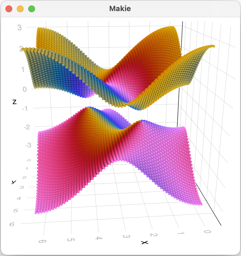
Lattice and bandstructure of a Kane-Mele model in graphene

julia> using Quantica, GLMakie, ProgressMeter

julia> SOC(dr) = ifelse(iseven(round(Int, atan(dr[2], dr[1])/(pi/3))), im, -im); # Kane-Mele spin-orbit coupling

julia> model = hopping(1, range = 1/√3) + @hopping((r, dr; α = 0) -> α * SOC(dr); sublats = :A => :A, range = 1) - @hopping((r, dr; α = 0) -> α * SOC(dr); sublats = :B => :B, range = 1);

julia> h = LatticePresets.honeycomb(a0 = 1) |> hamiltonian(model)
ParametricHamiltonian{Float64,2,2}: Parametric Hamiltonian on a 2D Lattice in 2D space
  Bloch harmonics  : 7
  Harmonic size    : 2 × 2
  Orbitals         : [1, 1]
  Element type     : scalar (ComplexF64)
  Onsites          : 0
  Hoppings         : 18
  Coordination     : 9.0
  Parameters       : [:α]

julia> qplot(h(α = 0.02), inspector = true)

julia> b = bands(h(α = 0.05), range(0, 2pi, length=60), range(0, 2pi, length = 60))
Bandstructure{Float64,3,2}: 3D Bandstructure over a 2-dimensional parameter space of type Float64
  Subbands  : 2
  Vertices  : 7200
  Edges     : 21122
  Simplices : 13924

julia> qplot(b, color = (psi, e, k) -> angle(psi[1] / psi[2]), colormap = :cyclic_mrybm_35_75_c68_n256, hide = :wireframe)

Fermi surface of a simple 3D cubic lattice

julia> pts = subdiv(0, 2π, 41); b = LP.cubic() |> hopping(1) |> bands(pts, pts, pts)
Bandstructure{Float64,4,3}: 4D Bandstructure over a 3-dimensional parameter space of type Float64
  Subbands  : 1
  Vertices  : 68921
  Edges     : 462520
  Simplices : 384000

julia> qplot(b[(:, :, :, 0.2)], hide = (:nodes, :wireframe))

Local density of states (LDOS) of a star-shaped mesoscopic cavity

julia> h = LP.square() |> onsite(4) - hopping(1) |> supercell(region = r -> norm(r) < 40*(1+0.2*cos(5*atan(r[2],r[1]))));

julia> g = h|> greenfunction;

julia> ρ = ldos(g(0.1 + 0.001im))
LocalSpectralDensitySolution{Float64} : local density of states at fixed energy and arbitrary location
  kernel   : LinearAlgebra.UniformScaling{Bool}(true)

julia> qplot(h, hide = :hops, sitecolor = ρ, siteradius = ρ, minmaxsiteradius = (0, 2), sitecolormap = :balance)

Four-terminal Green function and conductance

julia> hcentral = LP.square() |> hopping(-1) |> supercell(region = RP.circle(100) | RP.rectangle((202, 50)) | RP.rectangle((50, 202)))

julia> glead = LP.square() |> hopping(-1) |> supercell((1, 0), region = r -> abs(r[2]) <= 50/2) |> greenfunction(GS.Schur(boundary = 0));

julia> Rot = r -> SA[0 -1; 1 0] * r;  # 90º rotation function

julia> g = hcentral |>
           attach(glead, region = r -> r[1] ==  101) |>
           attach(glead, region = r -> r[1] == -101, reverse = true) |>
           attach(glead, region = r -> r[2] ==  101, transform = Rot) |>
           attach(glead, region = r -> r[2] == -101, reverse = true, transform = Rot) |>
           greenfunction;

julia> gx1 = sum(abs2, g(-3.96)[siteselector(), 1], dims = 2);

julia> qplot(hcentral, hide = :hops, siteoutline = 1, sitecolor = (i, r) -> gx1[i], siteradius = (i, r) -> gx1[i], minmaxsiteradius = (0, 2), sitecolormap = :balance)

julia> G₁₁ = conductance(g[1,1])
Conductance{Float64}: Zero-temperature conductance dIᵢ/dVⱼ from contacts i,j, in units of e^2/h
  Current contact  : 1
  Bias contact     : 1

julia> ωs = subdiv(-4, 4, 201); Gω = @showprogress [G₁₁(ω) for ω in ωs];
Progress: 100%|██████████████████████████████████████████████████████████████| Time: 0:01:01

julia> f = Figure(); a = Axis(f[1,1], xlabel = "eV/t", ylabel = "G [e²/h]"); lines!(a, ωs, Gω); f

[Datseris]

Amazing, this brings me back all the way to my PhD days were I was using Python’s Kwant (calling it from Julia)! Congratulations on the release! How much of Kwant’s capabilities does Quantica.jl implement? It appears they have similar target applications at least.

I was doing Landauer-Buttiker approach connecting leads to graphene microstructures and getting the scattering wavefunctions at each point on the lattice.

[pablosanjose]

Hey George, yes, Quantica’s scope and capabilities are rather similar to Kwant (although I haven’t used Kwant myself, to be honest). As far as I understand the approach is rather different, however, since Kwant is focused on 1D leads coupled to central systems (right?), while Quantica can mix systems of any dimensionality and use a variety of solvers for each part. Quantica is based on Green’s functions as the central object of interest, instead of Kwant’s scattering approach (although there is a mapping between the two, of course).

[garrek]

This is very cool! I’m excited whenever I see a new physics simulation package. I will be trying this to simulate some monolayer materials our group is using.

[pablosanjose]

That’s great @garrek. We are very much invested in developing Quantica further. Do let us know if you find any issue or lacking functionality. Bug reports are very welcome!

[pablosanjose]

Here is a recorded demo of Quantica.jl v1.0 with a more detailed walkthrough of features. It is a zoom presentation for the Quantum Tinkerer group (developers of Python’s kwant). They kindly game me permission to share it.

Quantica.jl demo, presented at the Quantum Tinkerer group (TUDelft)