Using MTK when I *import* ModelingToolkit?

[BLI]

Perhaps a silly question… As far as I know, ModelingToolkit.jl does not directly support quantities with units. In other words, I can not write something like (using Unitful.jl syntax…):

@component function MyModel(; name, struct_p = false, kwargs...)
    vars = @variables begin
        x(t)=1u"m"
        y(t)=2u"K"
    end

Instead, it is possible to write:

 vars = @variables begin
        x(t)=1,     [unit=u"m"]
        y(t)=2,     [unit=u"K"]
 end

or something to that effect. But this only works if SI units are provided…

Question: Would the following work?

 vars = @variables begin
        x(t)=ustrip(uconvert(u"m", 25u"in"),     [unit=u"m"]
        y(t)=ustrip(uconvert(u"K", 300u"°C"),     [unit=u"K"]
 end

The idea is to use the unit system of Unitful.jl to avoid conversion errors, but then strip off the unit in the assignment x(t) = , etc.

If this works, would it have a negative effect on performance?

[cryptic.ax]

That will work. As long as the default for the variable is unitless, and the unit given in the metadata is an SI unit, it is equivalent to you having done the conversion manually.

While we’re on the topic of units, Unitful.jl support is disappearing too. We support DynamicQuantities.jl, and it should be a drop-in replacement. The reason for the discontinuation is that Unitful.jl invalidates a lot of code, which prevents us from precompiling core workflows in MTK (a lot of work has gone into reducing TTFX). The validation for Unitful.jl was also subpar iirc.

[BLI]

My impression is that DynamicQuantities is more efficient than Unitful, but the documentation of Unitful is much more complete. There is some discussion in the DynamicQuantities documentation about being able to convert to/from Unitful, but it is not clear whether DynamicQuantities supports all units and constants in the Unitful package.

Anyways, my guess is that if I do as I indicate, and even drop specifying unit, this should work. And hopefully, using Unitful with conversion and stripping off units in the @parameters and @variables section does not influence the speed of the solver – since I assume that those sections are not used in the solver??

[cryptic.ax]

Unitful puts the units in the type. Theoretically, this means that if you have inconsistent units in your calculation the error is inferred at compile time. In practice, this doesn’t work out for MTK since we do the unit checking at model building time. The ODEProblem doesn’t have units in it. So putting things in the type only makes everything slower because everything ends up being a dynamic dispatch. DynamicQuantities puts the unit in the value domain, so it’s generally easier to work with.

[cryptic.ax]

Effectively, any concrete number you give to MTK should not have a unit. All units should be specified via the unit metadata. i.e. @variables x(t) = 1 [unit = u"m"] is fine, @variables x = 1u"m" is bad.

[BLI]

Got it. And even if I don’t want to use units (i.e., do not specify unit), I can convert to any non-SI unit, e.g.,

vars = @variables begin
        x(t)=ustrip(uconvert(u"mm", 25u"in"))
        y(t)=ustrip(uconvert(u"pK", 300u"°C"))
 end

and as long as I strip off units, there is no computational cost, even when I use Unitful over DynamicQuantities.

[BLI]

@cryptic.ax

As an example, the above form is pretty close to the @mtkmodel equivalent.

I’m struggling with how to include @structural_parameters in the new “MTK-model”.

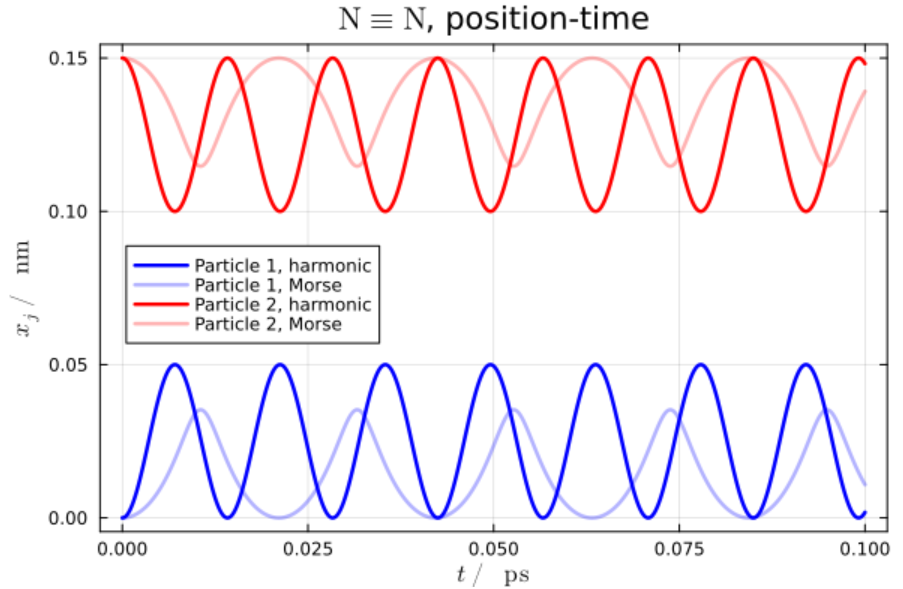
Here is a semi-realistic model [simulating 2 nitrogen atoms interacting via a harmonic and a Morse potential…].

My old/working model:

@mtkmodel TwoAtoms begin
    #
   # Model parameters
    # -- structure parameters
    @structural_parameters begin
        # typeP, :harmonic -- harmonic potential
        # typeP, :Morse -- Morse potential
        typeP = :harmonic
    end
    #
    # -- parameters
    #
    # Model parameters
    @parameters begin
        # Constant
        mb = 14,        [description = "Nitrogen atom mass, atom mass unit u"]
        D_e = 945,      [description = "Morse parameter D_e, unit u*nm^2/ps^2"]
        a = 27,         [description = "Morse parameter a, unit 1/nm"]
        r_e = 0.1,      [description = "Potential equilibrium distance, unit nm"]
        k_e = 2a^2*D_e, [description = "Harmonic parameter, u/ps^2"]
        r_0 = 1.5r_e,   [description = "Initial distance between particles, nm"]
        #
    end
    #
    # Model variables, with initial values needed
    @variables begin
        # Variables
        x_1(t)=0,           [description = "Particle 1, position unit nm"]
        v_1(t)=0,           [description = "Particle 1, velocity unit nm/ps"]
        x_2(t)=r_0,         [description = "Particle 2, position unit nm"]
        v_2(t)=0,           [description = "Particle 2, velocity unit nm/ps"]
        r(t),               [description = "Distance between particles, nm"]
        P(t),               [description = "Potential energy, u*nm^2/ps^2"]
        K(t),               [description = "Kinetic energy, u*nm^2/ps^2"]
        E(t),               [description = "Total energy, u*nm^2/ps^2"]
    end
    #
    # Model equations
    @equations begin
        # Basic algebraics
        K ~ mb*(v_1^2 + v_2^2)/2
        r ~ abs(x_1 - x_2)
        #
        # Velocity definitions
        Dt(x_1) ~ v_1
        Dt(x_2) ~ v_2
        # Dynamics based on typeP
        if typeP == :harmonic  
            Dt(v_1) ~ -k_e*(r - r_e)*sign(x_1-x_2)/mb
            Dt(v_2) ~ k_e*(r - r_e)*sign(x_1-x_2)/mb
            P ~ k_e/2*(r-r_e)^2
        elseif typeP == :Morse
            Dt(v_1) ~ -2*D_e*a*(1-exp(-a*(r-r_e)))*exp(-a*(r-r_e))*sign(x_1-x_2)/mb
            Dt(v_2) ~ 2*D_e*a*(1-exp(-a*(r-r_e)))*exp(-a*(r-r_e))*sign(x_1-x_2)/mb
            P ~ D_e*(1 - exp(-a*(r-r_e)))^2
        end
        E ~ K + P
    end
end

and here is how I instantiate two models:

@mtkcompile tp_h = TwoAtoms()
@mtkcompile tp_m = TwoAtoms(;typeP=:Morse)

---

Next, I am trying to use the @component macro, but do not understand how to handle structural_parameters. Here is the same code as above, where I have had to comment out the structural parameter typeP in order to make it work:

@component function TwoAtomsNew(; name)
    #
   # Model parameters
    # -- structure parameters
    #=
    struct_params = @structural_parameters begin
        # typeP, :harmonic -- harmonic potential
        # typeP, :Morse -- Morse potential
        typeP = :harmonic
    end
    =#
    #
    # -- parameters
    #
    # Model parameters
    params = @parameters begin
        # Constant
        mb = 14,        [description = "Nitrogen atom mass, atom mass unit u"]
        D_e = 945,      [description = "Morse parameter D_e, unit u*nm^2/ps^2"]
        a = 27,         [description = "Morse parameter a, unit 1/nm"]
        r_e = 0.1,      [description = "Potential equilibrium distance, unit nm"]
        k_e = 2a^2*D_e, [description = "Harmonic parameter, u/ps^2"]
        r_0 = 1.5r_e,   [description = "Initial distance between particles, nm"]
        #
    end
    #
    # Model variables, with initial values needed
    vars = @variables begin
        # Variables
        x_1(t)=0,           [description = "Particle 1, position unit nm"]
        v_1(t)=0,           [description = "Particle 1, velocity unit nm/ps"]
        x_2(t)=r_0,         [description = "Particle 2, position unit nm"]
        v_2(t)=0,           [description = "Particle 2, velocity unit nm/ps"]
        r(t),               [description = "Distance between particles, nm"]
        P(t),               [description = "Potential energy, u*nm^2/ps^2"]
        K(t),               [description = "Kinetic energy, u*nm^2/ps^2"]
        E(t),               [description = "Total energy, u*nm^2/ps^2"]
    end
    #
    # Model equations
    eqs = [
        # Basic algebraics
        K ~ mb*(v_1^2 + v_2^2)/2
        r ~ abs(x_1 - x_2)
        #
        # Velocity definitions
        Dt(x_1) ~ v_1
        Dt(x_2) ~ v_2
        # Dynamics based on typeP
        #if typeP == :harmonic  
            Dt(v_1) ~ -k_e*(r - r_e)*sign(x_1-x_2)/mb
            Dt(v_2) ~ k_e*(r - r_e)*sign(x_1-x_2)/mb
            P ~ k_e/2*(r-r_e)^2
        #=elseif typeP == :Morse
            Dt(v_1) ~ -2*D_e*a*(1-exp(-a*(r-r_e)))*exp(-a*(r-r_e))*sign(x_1-x_2)/mb
            Dt(v_2) ~ 2*D_e*a*(1-exp(-a*(r-r_e)))*exp(-a*(r-r_e))*sign(x_1-x_2)/mb
            P ~ D_e*(1 - exp(-a*(r-r_e)))^2
        end 
        E ~ K + P =#
    ]
    #
    System(eqs, t, vars, params; name)
end

Instantiating this new version works by doing:

@mtkcompile tp_h = TwoAtomsNew()

Question: How can I extend TwoAtomsNew with the structural parameter?

[baggepinnen]

Try this

    eqs = [
        # Basic algebraics
        K ~ mb*(v_1^2 + v_2^2)/2
        r ~ abs(x_1 - x_2)
        # Velocity definitions
        Dt(x_1) ~ v_1
        Dt(x_2) ~ v_2
        # Dynamics based on typeP
        if typeP == :harmonic  
            [Dt(v_1) ~ -k_e*(r - r_e)*sign(x_1-x_2)/mb
            Dt(v_2) ~ k_e*(r - r_e)*sign(x_1-x_2)/mb
            P ~ k_e/2*(r-r_e)^2]
        elseif typeP == :Morse
            [Dt(v_1) ~ -2*D_e*a*(1-exp(-a*(r-r_e)))*exp(-a*(r-r_e))*sign(x_1-x_2)/mb
            Dt(v_2) ~ 2*D_e*a*(1-exp(-a*(r-r_e)))*exp(-a*(r-r_e))*sign(x_1-x_2)/mb
            P ~ D_e*(1 - exp(-a*(r-r_e)))^2]
        end 
        E ~ K + P
    ]

That is, each branch of the if statement returns an array that is then concatenated with the rest of the equations. This is not MTK specific, it works for any julia code

julia> [
       1
       2
       if true
         [3,4]
       else
         [5,6]
       end
       7
       ]
5-element Vector{Int64}:
 1
 2
 3
 4
 7

[BLI]

How do I introduce typeP?

There appears to be no “macro” @structural_parameters for @component.

Should I do:

@component function TwoAtomsNew(; name, typeP=:harmonic)

---

OK – tested it, and it works. Thanks!

[baggepinnen]

@BLI

There appears to be no “macro” @structural_parameters for @component.

Correct, a structural parameter is just a function argument that isn’t used to create a symbolic variable.

[BLI]

And… here is the result when using @component – the same as when using the old system:

[BLI]

Ah. I ran into another problem… suppose I use a structural parameter to decide whether I should leave an input perturbation as zero or undefined (for the purpose of linearization). Here is a basic example:

@component function SimpleSys(; name, u_ex=false)
    #
   # Model parameters
    # -- structure parameters
        # u_ex, false -- no input perturbation
        # u_ex, true -- input perturbation is undefined
    #
    # -- parameters
    #
    # Model parameters
    params = @parameters begin
        a = -2
        b = 0.5
        #
    end
    #
    # Model variables, with initial values needed
    # Variables
    vars = @variables begin
        x(t) = 3.0
        y(t) = 1.0
        u(t) = 0.0
        du(t)
    end
    #
    # Model equations
    eqs = [
        u ~ 1
        if u_ex == false
            du ~ 0
        end
        Dt(x) ~ a*x + b*(u+du)
        Dt(y) ~ -x + 2*a*y
    ]
    #
    System(eqs, t, vars, params; name)
end

I can instantiate this:

@mtkcompile sisy = SimpleSys()

Next, I try to set u_ex = true, which means that I want an “external” input du that is unspecified:

@named sisy_lin = SimpleSys(; u_ex=true)
sisy_lin = complete(sisy_lin)

The idea is that sisy_lin has an unspecified input du which I can use in linearization.

This worked in the past, but does not work now.

Question: what has changed?

[baggepinnen]

@BLI

suppose I use a structural parameter to decide whether I should leave an input perturbation as zero or undefined (for the purpose of linearization).

You shouldn’t We have a mechanism called “analysis point” to handle exactly this issue. Always connect it, but connect it like this

connect(y, :name, u)

and then when you want to linearize, you pass sys.name instead of u as the input, and the connection will be removed automatically.

[BLI]

Yes, I know about the “analysis point”. My guess is that it does more or less what I have indicated, i.e., create an extra “fictitious” input that is set to zero for normal simulation. Then during “analysis”, this value is relaxed from zero and used as the input during linearization if it is an input in the linearization – this makes it trivial to choose the operating point value for this “fictitious” input, and is kept as an output otherwise.

---

The only “disadvantage” with using “analysis point” is that I think it is necessary to:

• Add the ModelingToolkitStandardLibrary [not a disadvantage in itself, of course, but adds complexity)
• Add components from ModelingToolkitStandardLibrary for “input signal” and “output signal” (?) and connect these as you indicate. Again, not a disadvantage per se, but adds some complexity.

For the “old” way of defining the model, I could simply do:

@mtkmodel SimpleSys begin
   # Model parameters
    # -- structure parameters
    @structural_parameters begin
        # u_ex, boolean, input U defined EXternally
        u_ex = false
    end
    #
    # Model parameters
    @parameters begin
        a = -2
        b = 0.5
        #
    end
    #
    # Model variables, with initial values needed
    # Variables
    @variables begin
        x(t) = 3.0
        y(t) = 1.0
        u(t) = 0.0
        du(t)
    end
    #
    # Model equations
   @equations begin
        u ~ 1
        if u_ex == false
            du ~ 0
        end
        Dt(x) ~ a*x + b*(u+du)
        Dt(y) ~ -x + 2*a*y
    end
end

and

@named sisy_lin = SimpleSys(; u_ex=true)
sisy_lin = complete(sisy_lin)

and it worked.

---

Is there an updated example with new @component macro with RealInput etc. from MTKSL, etc. that works?

[baggepinnen]

This works

Dt = ModelingToolkit.D_nounits
t = ModelingToolkit.t_nounits
@mtkmodel SimpleSys2 begin
   # Model parameters
    # -- structure parameters
    @structural_parameters begin
        # u_ex, boolean, input U defined EXternally
        u_ex = false
    end
    #
    # Model parameters
    @parameters begin
        a = -2
        b = 0.5
        #
    end
    #
    # Model variables, with initial values needed
    # Variables
    @variables begin
        x(t) = 3.0
        y(t) = 1.0
        u(t)# = 0.0
        du(t), [input = true]
        c0(t), [output = true]
    end
    #
    # Model equations
   @equations begin
        u ~ 1
        c0 ~ 0
        connect(c0, :name, du)
        Dt(x) ~ a*x + b*(u+du)
        Dt(y) ~ -x + 2*a*y
    end
end

@named model = SimpleSys2()
linearize(model, [model.name], [])

you no longer need MTKStdlib to use analysis points, declarig variables as input/output as above is sufficient

[BLI]

Great that the analysis point idea has been incorporated into MTK itself!

A couple of things in the example SimpSys2 that I don’t quite get.

You introduce c0 as an output, and then give it a value of 0.

• Is this meant to be the “output” of an external input signal that functions as an additional input to the system?

Then you connect c0 to du.

• Does this mean that you give du the value of c0 by connecting them, but you add the possibility of the analysis point?
• What precisely does this analysis point do? Does it add a hidden variable (that the user does not need to know about), say named du_p or something (p for perturbation) which is set to zero for normal simulation, but that is allowed to be different from zero during linearization and with zero operating point?

What does linearize do?

• linearize(model, [model.name], []) … it linearizes from the analysis point (model.name)… to what output? To all states when an output is not listed?

[baggepinnen]

@BLI

You introduce c0 as an output, and then give it a value of 0.

• Is this meant to be the “output” of an external input signal that functions as an additional input to the system?

There’s a rule that connect between two variables is only allowed if one is an input and the other is an output.

@BLI

Does this mean that you give du the value of c0 by connecting them, but you add the possibility of the analysis point?

correct

@BLI

What precisely does this analysis point do?

it depends on how you’re using it. When you simulate the model it does nothing, when you call linearize it performs a number of model transformations. I’ll plan to submit a talk on this on the upcoming MODPROD conference in a few months, but I haven’t yet put the material together. In this case, it breaks the connection (like it wasn’t there), adds a new virtual input that is connected to the input variable in the connection and uses this new virtual input as the linearization input.

If you call get_looptransfer, get_sensitivity etc., the analysis point does other things, as appropriate to give you the requested function.

@BLI

linearize(model, [model.name], []) … it linearizes from the analysis point (model.name)… to what output? To all states when an output is not listed?

In this case I listed no outputs, so the C matrix is empty. You still get the A,B matrices though.

[BLI]

So I re-wrote your working code to the new @Component syntax, and simplified it + slight change of notation:

# Dt = ModelingToolkit.D_nounits
# t = ModelingToolkit.t_nounits
@component function SimpleSys3(; name)
   # Model parameters
    #
    # Model parameters
    params = @parameters begin
        a = -2
        b = 0.5
        #
    end
    #
    # Model variables, with initial values needed
    # Variables
    vars = @variables begin
        x(t) = 3.0
        z(t) = 1.0
        u(t), [input = true]
        u_ex(t), [output = true]
    end
    #
    # Model equations
   eqs = [
        u_ex ~ 1
        connect(u_ex, :pump, u)
        Dt(x) ~ a*x + b*u
        Dt(z) ~ -x + 2*a*z
   ]
   #
   System(eqs,t,vars,params; name)
end

@named model3 = SimpleSys3()

linearize(model3, [model3.pump], [])

This works. But what if I want to specify the output in the linearization? Suppose I want to do y ~ z and use y as output leading to C and D matrices.

Doing:

linearize(model3, [model3.pump], [model3.z])

does not work.

[baggepinnen]

Use complete(model).z for the output. It’s unfortunate that this discrepancy exists, but I think @cryptic.ax has some explanation for why it’s hard to get rid of.

[BLI]

Ah. I think I figured it out. I needed to re-wire my brain

• I am used to thinking in terms of linearization from an input signal to a system, to an output signal from the system.
• But with “analysis points”, I must instead think in terms of linearization from one connection point to another connection point.
• Connection points are defined by connectors between components.

In my simple example above, at the outset, that is the only component there is, and there is no component upstream or downstream in the information flow.

So I need to create fictitious upstream and downstream “components”. In my example above, u_ex is actually the output signal from the upstream “component”, so I rename it to y_up. Then I must connect that “output” from the upstream “component” to the input u of the model/component I describe here.

---

OK. To define a downstream connection, I need to treat the output y from my system as an output from this “component”, and then I need to add u_dwn as an input to the fictitious downstream component. And finally make a connection seemingly outside of my model by connecting the output y of this model to the fictitious input u_dwn of the downstream system.

# Dt = ModelingToolkit.D_nounits
# t = ModelingToolkit.t_nounits
@component function SimpleSys3(; name)
   # Model parameters
    #
    # Model parameters
    params = @parameters begin
        a = -2
        b = 0.5
        #
    end
    #
    # Model variables, with initial values needed
    # Variables
    vars = @variables begin
        x(t) = 3.0
        z(t) = 1.0
        u(t), [input = true]
        y_up(t), [output = true]
        y(t), [output = true]
        u_dwn(t), [input = true]

    end
    #
    # Model equations
   eqs = [
        y_up ~ 1
        connect(y_up, :pump, u)
        Dt(x) ~ a*x + b*u
        Dt(z) ~ -x + 2*a*z
        y ~ z 
        connect(y, :sensor, u_dwn)
   ]
   #
   System(eqs,t,vars,params; name)
end

@named model3 = SimpleSys3()
linsys = linearize(model3, [model3.pump], [model3.sensor])

In summary, although I really only have a single system that is not even a component, I need to treat it as a component and define u as input, and y as output.

In addition, I need to create a “fictitious” upstream component with output y_up, and a fictitious downstream component with input u_dwn.

Then I do the “component” connections with analysis points.

---

Does this seem correct?