Solving for transcendental equation

Hi,

I have the function f_n(x) = e^x T_n(x), where T_n are Touchard’s polynomials. The function is bijective from R to R and everything is Ok, just that the inverse is unknown… It has the nice taylor exapnsion :

f_n(x) = \sum_{k \in \mathbb N} k^n \frac{x^k}{k!}.

For the moment I am using root solving, but since this happens in a very hot loop, I’d like to do better and somehow precompute a polynomial expansion for the inverse, or something else maybe ? I have the following code that implements the function for the moment:

using Roots

function fₙ(x, ::Val{n}) where n
    n==1 && return exp(x)
    t = zeros(n)
    # recurence to compute stirling numbers, the coeficients of touchard's polynomials: 
    t[1] = 1
    for j in 2:n
        t[2:j] .= t[1:j-1] .+ collect(2:j) .* t[2:j]
    end 
    return sum(t .* x.^(1:n)) * exp(x)
end
function inv_fₙ(x, ::Val{n}) where n
    n==1 && return log(x)
    fzero(t -> fₙ(t, Val{n}())-x, 0)
end

inv_fₙ(3, Val{2}()) # This is the set of function that i want to interpolate. 

This isnt very efficient since the coefficients could be stored instead of recomputed each time, moreover with allocations, but my concern is on making the inverse function efficient, not this one :slight_smile:

Is there tools in Julia to construct a pre-boiled-down representation of an inverse function ? polynomial interpolation ? something else ?

If you want this on a finite domain, Remez.jl is pretty good (although the UI definitely isn’t ideal). I think ApproxFun.jl or FastChebInterp.jl may be useful to you (but I haven’t used either)

1 Like

Nope, sadly i need it on \mathbb R_+. Is it theoreticaly an issue ?

Not an issue, just means you probably want to use one of the 2nd or 3rd options.

Ok, I have the following:

using Roots

function fₙ(x, ::Val{n}) where n
    n==1 && return exp(x)
    t = zeros(n)
    # recurence to compute stirling numbers, the coeficients of touchard's polynomials: 
    t[1] = 1
    for j in 2:n
        t[2:j] .= t[1:j-1] .+ collect(2:j) .* t[2:j]
    end 
    return sum(t .* x.^(1:n)) * exp(x)
end
function inv_fₙ(x, ::Val{n}) where n
    n==1 && return log(x)
    fzero(t -> fₙ(t, Val{n}())-x, 1)
end

using ApproxFun


f1 = log
f2 = Fun(x -> inv_fₙ(x, Val{2}()), Laguerre())
f3 = Fun(x -> inv_fₙ(x, Val{3}()), Laguerre())
f4 = Fun(x -> inv_fₙ(x, Val{4}()), Laguerre())

using Plots
x = 0:0.1:20
plot(x, f1.(x), label="n=1")
plot!(x, f2.(x), label="n=2")
plot!(x, f3.(x), label="n=3")
plot!(x, f4.(x), label="n=4")

which gives:

but then if i try to increase the scope

x = 0:0.1:100
plot(x, inv_fₙ.(x, Val{2}()))
plot!(x, f2.(x), label="n=2")

there are artefacts:

Since these functions look very smooth and regular, maybe the Laguerre basis is not the right one. Maybe someone has a better idea ?

  1. Since fzero calls f_n with the same n, computing the t array once and reusing it on the next calls from fzero would increase speed substantially.

  2. Another suggestion is to use Newton’s method in find_zero, based on the available analytic form of the derivative:

d f_n(x)/dx = f_(n+1)(x) / x - 1

  1. Use find_zero instead of fzero. As evidenced by docs and experiment, find_zero specializes on function argument and thus speeds up repeated calls to argument. Benchmark shows substantial improvement.

Benchmark the following:

using Combinatorics, Roots

function fₙ4(x, ::Val{n}, s2::NTuple{n, Int}) where n
    n==1 && return exp(x)
    return sum(s2 .* x.^(1:n)) * exp(x)
end

function inv_fₙ4(x, ::Val{n}) where n
    n==1 && return log(x)
    return find_zero(
      let s2 = ntuple(i->stirlings2(n, i), n)
          t -> fₙ4(t, Val{n}(), s2)-x
      end, 0.0)
end
1 Like

It may be beneficial to split your domain up into 2 portions: [0, k] and [k, inf], and then deal with the 2nd by approximating inv_fₙ(1/x) on (0, 1/k].

1 Like

Laguerre() uses unweighted Laguerre polynomials as the basis. It will always blow up at infinity. You probably want WeightedLaguerre(), which uses the exponentially weighted polynomials (unfortunately not properly documented, but it’s there).

1 Like

Isn’t it be easier to use something like atanh to map the interval to something finite, e.g. approximate inv_fₙ(atanh(x)) on [0,1]? Or does that produce numerical problems?

1 Like

x = \frac{t}{1 - t} is a common substitution for such purposes, see for example Examples · QuadGK.jl.

I can’t quote literature or give a rigorous explanation, but I’ve found that an algebraic substitution like that usually behaves a bit better than a logarithmic one like -log1p(-t) or atanh(t), because the latter grow fairly slowly, so to get even moderately large x, your t has to be incredibly close to 1. In other words, a reasonable set of sample points in [0, 1], such as Chebyshev or Legendre nodes, could easily miss important large-x behavior on [0, \infty) when using a logarithmic substitution, which would be sampled (albeit sparsely) using the algebraic substitution. I guess this is less relevant if you know a priori that the function you’re trying to approximate decays exponentially.

1 Like

the two nice things about a 1/x` transform are that it’s easy to compute, and the item is a good series of that form that converges well.

1 Like

Oh one other thing is that it might make sense to try generating the exponential of the inverse function rather than the inverse itself.

hum…

The 1/(1+x) ↔ t/(1-t) mapping fails the root solver somehow, the 1/x mapping reaches the maximum number of coefficients ApproxFun takes, and the WeightedLaguerre never terminates…

I’m using @Dan’s version now:

using Roots, Combinatorics, ApproxFun, Plots

function fₙ(x, ::Val{n}, s2::NTuple{n, Int}=ntuple(i->stirlings2(n, i), n)) where n
    n==1 && return exp(x)
    return sum(s2 .* x.^(1:n)) * exp(x)
end
function inv_fₙ(x, ::Val{n}) where n
    n==1 && return log(x)
    return find_zero(
      let s2 = ntuple(i->stirlings2(n, i), n)
          t -> fₙ(t, Val{n}(), s2)-x
      end, (0.0,Inf))
end


# This reaches millions of coefficients somehow:  
inv_fns = (log, (
    Fun(x -> inv_fₙ(x/(1-x), Val{k}()), Interval(0,1)) ∘ (x -> x/(1+x)) for k in 2:5
)...)

# This also reaches millions: 
first_part = (log, (
        Fun(x -> inv_fₙ(x, Val{k}()), Interval(0,k)) for k in 2:5
)...)
second_part = (log, (
    Fun(x -> inv_fₙ(1/x, Val{k}()), Interval(0,k)) ∘ inv for k in 2:5
)...)

# WHile this never terminates: 
inv_fns = (log, (
    Fun(x -> inv_fₙ(x, Val{k}()), WeightedLaguerre()) for k in 2:5
)...)

Dunno what to try next :confused:


Edit: I was able to restrict the root search using the folloiwng upper bound:

x = 0.0001:0.1:20
p = plot(x, max.(log(2), log.(x)), label="upper bound log(x ∧ 2)")
for k in 2:10
    plot!(p, x, inv_fₙ.(x, Val{k}()), label="n=$k")
end
p

Since your root finding is monotonic, and you can get decent bounds, you might want to try IntervalNonlinearProblemfrom BracketingNonlinearSolve.jl (one of the sub-libraries of NonlinearSolve.jl. By bracketing your function with a sign change, you get to use some really fast solvers (the default is ITP which is quite good). Also, log1p is a cleaner and tighter upper bound than max(log(2), 2log(x))

You’ll also get faster and more stable fₙ computation by using evalpoly.

function fₙ(x, ::Val{n}, s2::NTuple{n, Int}=ntuple(i->stirlings2(n, i), n)) where n
    n==1 && return exp(x)
    return x*evalpoly(x, s2) * exp(x)
end
function inv_fₙ(x, ::Val{n}) where n
    n==1 && return log(x)
    s2 = ntuple(i->stirlings2(n, i), n)
    prob = IntervalNonlinearProblem{false}((t, s2) -> fₙ(t, Val{n}(), s2)-x,
       (0.0, log1p(x)),
       s2)
    solve(prob).u
end
3 Likes

With all of this,

inv_fns = (log, (
           Fun(x -> inv_fₙ(x/(1-x), Val{k}()), Interval(1e-6,1-1e-6)) ∘ (x -> x/(1+x)) for k in 2:5
       )...)

works. You can’t quite push the bounds to 0 or 1 (since at 0 it’s infinitely steep, and at 1 you’re evaluating inv_fₙ at infinity).

1 Like

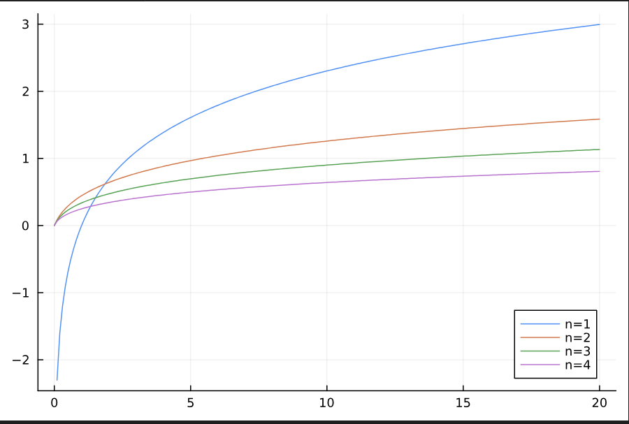
Thanks a lot to everyone, i have working things now. However, from the begining the problem was not the right one, I am realizing now that the part of the curve I need to invert is not

f_n: \mathbb R_+ \to \mathbb R

but rather

f_n: [-\infty, x_n^*] \to \mathbb R_+ \text{ if n even, and } f_n: [-\infty, y_n^*] \to \mathbb R_- \text{ when n odd},

where x^* is the leftmost critical point of f_n, that is the leftmost root of its derivative.
Since f_n' = f_{n+1} / (x-1), that is the leftmost root of f_{n+1}. All roots of touchard’s polynomials are real and negatives.

Since this is the leftmost one, the part where i need to do the grid search is still monotonous so we are good. The issue is that I do not really know where is this leftmost root, even if wikipedia has a few hints.

Back to the drawing board I guess :rofl:


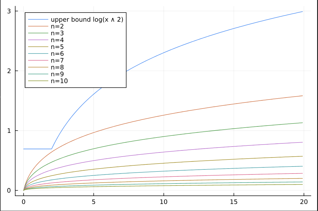
So Wikipedia gives a lower bound for the leftmost root :

So i guess that evaluating f_n at this lower bound would give a good starting point to look for the root. However, we should not go too far to the right and pass through the root, otherwise we are cooked (the function is not monotone there anymore). I will retry writing a solver.


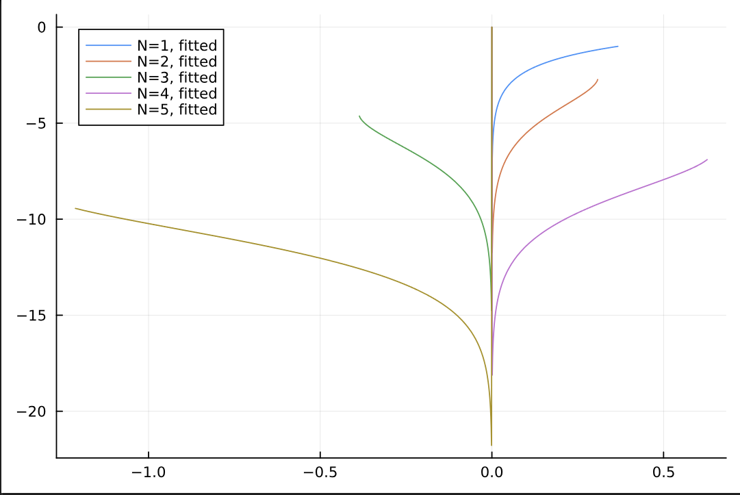
Here is a piece of code that reimplements the inverse function that i needed. The interpolation is working correctly, even if there are a few artefacts.

and this is what i obtain after interpolation:

Current code
using Roots, Combinatorics, ApproxFun, Plots

function fₙ(x, ::Val{n}, s2::NTuple{n, Int}=ntuple(i->stirlings2(n, i), n)) where n
    n==1 && return exp(x)
    return x*evalpoly(x, s2) * exp(x)
end

function lower_bound_on_leftmost_root(::Val{n}) where n
    n==2  && return - 1.0
    n==3  && return - 1 / 0.380
    n==4  && return - 1 / 0.216
    n==5  && return - 1 / 0.145
    n==6  && return - 1 / 0.106
    n==7  && return - 1 / 0.082
    n==8  && return - 1 / 0.066
    n==9  && return - 1 / 0.055
    n==10 && return - 1 / 0.046
    C2 = binomial(n, 2)
    C3 = binomial(n, 3)
    C4 = binomial(n, 4)
    term1 = C2 / n
    discr = C2^2 - (2n / (n - 1)) * (C3 + 3*C4)
    term2 = (n - 1)/n * sqrt(discr)
    lower_bound = (term1 + term2)
    return -lower_bound
end

leftmost_critical_point(::Val{n}) where n = lower_bound_on_leftmost_root(Val{n+1}())
starting_point(::Val{n}) where n = leftmost_critical_point(Val{n+1}())
last_summit(::Val{n}) where n = fₙ(leftmost_critical_point(Val{n}()), Val{n}())

function inv_fₙ(x, ::Val{n}) where n
    n==1 && return log(x)
    x₀ = starting_point(Val{n}())
    return find_zero(
      let s2 = ntuple(i->stirlings2(n, i), n)
          t -> fₙ(t, Val{n}(), s2)-x
      end, 
      x₀
      )
end

N=3
x = -10:0.1:0
plot(x, fₙ.(x, Val{N}()))

lower_bound_on_leftmost_root(Val{N}())

leftmost_critical_point(Val{N}())

# The range of the inverse will be [summit,0] or [0,summit] depending on the usmmit sign (summit is neg is N is odd and pos is N is even i think)
last_summit(Val{N}())


starting_point(Val{N}())

inv_fₙ(-0.1, Val{N}())

N=1
s = last_summit(Val{N}())
x = sign(s) .* (1e-5:0.001:abs(s))
plot(x, inv_fₙ.(x, Val{N}()), label="N=$N, truth")
# I think this one should be the lambert W function as f_1 = e^x * x IIRC. 

N=2
s = last_summit(Val{N}())
x = sign(s) .* (1e-5:0.001:abs(s))
plot!(x, inv_fₙ.(x, Val{N}()), label="N=$N, truth")

N=3
s = last_summit(Val{N}())
x = sign(s) .* (1e-5:0.001:abs(s))
plot!(x, inv_fₙ.(x, Val{N}()), label="N=$N, truth")

N=4
s = last_summit(Val{N}())
x = sign(s) .* (1e-5:0.001:abs(s))
plot!(x, inv_fₙ.(x, Val{N}()), label="N=$N, truth")

N=5
s = last_summit(Val{N}())
x = sign(s) .* (1e-5:0.001:abs(s))
plot!(x, inv_fₙ.(x, Val{N}()), label="N=$N, truth")


function mkfun(::Val{n}) where n
    s = last_summit(Val{n}())
    I = s > 0 ? Interval(1e-4, s) : Interval(s, -1e-4)
    return Fun(x -> inv_fₙ(x, Val{n}()), I)
end

inv_fns = (log, (mkfun(Val{k}()) for k in 2:5)...)

plot()
for (n, f) in enumerate(inv_fns)
    s = last_summit(Val{n}())
    x = sign(s) .* (1e-5:0.001:abs(s))
    plot!(x, f.(x), label="N=$n, fitted")
end
plot!()

Does someone have an idea on how i could validate the result, and extract the polynomials from the objects to store them on disk somehow ?