Smooth approximation to max(0, x)

I need a “smooth” approximation f to x \to \max(0, x), such that

  1. \lim_{x \to -\infty} f(x) = 0,
  2. \lim_{x \to \infty} f(x) = x,
  3. f(x) > 0, f'(x) > 0, both continuous; ideally continuous higher derivatives
  4. not too expensive to calculate.

I am aware of \log(a + \exp(x)), which can be implemented with LogExpFunctions.log1pexp, is there anything else?

1 Like

Would you accept a function that approximates only around 0 and is exactly equal to 0 before a constant -a and to x after a constant b ? If so, we could provide a very efficient solution (in term of computational time) with e.g. a bezier curve

You mean a cubic polynomial matching the derivatives and the values at -a and b? I could try that, but I am looking for something smoother.

1 Like

Have you seen “mish” and “squareplus” from
Rectifier (neural networks) - Wikipedia, or the Smooth Maximum Unit?

This paper considers a number of smoothed functions When are smooth-ReLUs ReLU-like? | OpenReview

3 Likes

by pattern matching Id guess maybe anything that is invf(f(0) + f(x)) where f is increasing monotonically and has range (0,inf) ?? First guess is usually wrong tho

That’s a good pattern for sure. Similar to the “smooth absolute value” sqrt(x^2 + c)

I may be misunderstanding something, but that’s precisely the kind of function I am looking for. sure, if I have it, I can transform it a lot of ways.

No, but thanks, this is very helpful.

1 Like

Does \log(a + \exp(x)) have an unwanted property, or do you want to know other functions just in general?

2 Likes

How about:

t = (1/4)^(1/3)
t1, t2 = t^4 - t, t^4
julia> relu(x) = ifelse(x > 0, x, 0)
relu (generic function with 1 method)

julia> lineplot(-0.5,0.5,x-> t1 < x < t2 ? (x-t1)^4 : relu(x))
            ┌────────────────────────────────────────┐       
        0.5 │⠀⠀⠀⠀⠀⠀⠀⠀⠀⠀⠀⠀⠀⠀⠀⠀⠀⠀⠀⠀⡇⠀⠀⠀⠀⠀⠀⠀⠀⠀⠀⠀⠀⠀⠀⠀⠀⠀⢀⡞│ #57(x)
            │⠀⠀⠀⠀⠀⠀⠀⠀⠀⠀⠀⠀⠀⠀⠀⠀⠀⠀⠀⠀⡇⠀⠀⠀⠀⠀⠀⠀⠀⠀⠀⠀⠀⠀⠀⠀⠀⣀⠎⠀│       
            │⠀⠀⠀⠀⠀⠀⠀⠀⠀⠀⠀⠀⠀⠀⠀⠀⠀⠀⠀⠀⡇⠀⠀⠀⠀⠀⠀⠀⠀⠀⠀⠀⠀⠀⠀⠀⡰⠃⠀⠀│       
            │⠀⠀⠀⠀⠀⠀⠀⠀⠀⠀⠀⠀⠀⠀⠀⠀⠀⠀⠀⠀⡇⠀⠀⠀⠀⠀⠀⠀⠀⠀⠀⠀⠀⠀⠀⡖⠁⠀⠀⠀│       
            │⠀⠀⠀⠀⠀⠀⠀⠀⠀⠀⠀⠀⠀⠀⠀⠀⠀⠀⠀⠀⡇⠀⠀⠀⠀⠀⠀⠀⠀⠀⠀⠀⠀⢀⠎⠀⠀⠀⠀⠀│       
            │⠀⠀⠀⠀⠀⠀⠀⠀⠀⠀⠀⠀⠀⠀⠀⠀⠀⠀⠀⠀⡇⠀⠀⠀⠀⠀⠀⠀⠀⠀⠀⠀⡠⠃⠀⠀⠀⠀⠀⠀│       
            │⠀⠀⠀⠀⠀⠀⠀⠀⠀⠀⠀⠀⠀⠀⠀⠀⠀⠀⠀⠀⡇⠀⠀⠀⠀⠀⠀⠀⠀⠀⠀⡜⠁⠀⠀⠀⠀⠀⠀⠀│       
   f(x)     │⠀⠀⠀⠀⠀⠀⠀⠀⠀⠀⠀⠀⠀⠀⠀⠀⠀⠀⠀⠀⡇⠀⠀⠀⠀⠀⠀⠀⠀⢠⠏⠀⠀⠀⠀⠀⠀⠀⠀⠀│       
            │⠀⠀⠀⠀⠀⠀⠀⠀⠀⠀⠀⠀⠀⠀⠀⠀⠀⠀⠀⠀⡇⠀⠀⠀⠀⠀⠀⠀⡤⠃⠀⠀⠀⠀⠀⠀⠀⠀⠀⠀│       
            │⠀⠀⠀⠀⠀⠀⠀⠀⠀⠀⠀⠀⠀⠀⠀⠀⠀⠀⠀⠀⡇⠀⠀⠀⠀⠀⢀⡔⠁⠀⠀⠀⠀⠀⠀⠀⠀⠀⠀⠀│       
            │⠀⠀⠀⠀⠀⠀⠀⠀⠀⠀⠀⠀⠀⠀⠀⠀⠀⠀⠀⠀⡇⠀⠀⠀⠀⡠⠊⠀⠀⠀⠀⠀⠀⠀⠀⠀⠀⠀⠀⠀│       
            │⠀⠀⠀⠀⠀⠀⠀⠀⠀⠀⠀⠀⠀⠀⠀⠀⠀⠀⠀⠀⡇⠀⠀⢀⡔⠁⠀⠀⠀⠀⠀⠀⠀⠀⠀⠀⠀⠀⠀⠀│       
            │⠀⠀⠀⠀⠀⠀⠀⠀⠀⠀⠀⠀⠀⠀⠀⠀⠀⠀⠀⠀⡇⢀⡔⠃⠀⠀⠀⠀⠀⠀⠀⠀⠀⠀⠀⠀⠀⠀⠀⠀│       
            │⠀⠀⠀⠀⠀⠀⠀⠀⠀⠀⠀⠀⠀⠀⠀⠀⠀⠀⣀⡤⡗⠁⠀⠀⠀⠀⠀⠀⠀⠀⠀⠀⠀⠀⠀⠀⠀⠀⠀⠀│       
          0 │⣀⣀⣀⣀⣀⣀⣀⣀⣀⣀⣀⣀⣀⡤⠤⠔⠒⠋⠁⠀⡇⠀⠀⠀⠀⠀⠀⠀⠀⠀⠀⠀⠀⠀⠀⠀⠀⠀⠀⠀│       
            └────────────────────────────────────────┘       
            ⠀-0.5⠀⠀⠀⠀⠀⠀⠀⠀⠀⠀⠀⠀⠀⠀⠀⠀⠀⠀⠀⠀⠀⠀⠀⠀⠀⠀⠀⠀⠀⠀⠀⠀⠀0.5⠀       
            ⠀⠀⠀⠀⠀⠀⠀⠀⠀⠀⠀⠀⠀⠀⠀⠀⠀⠀⠀⠀⠀x⠀⠀⠀⠀⠀⠀⠀⠀⠀⠀⠀⠀⠀⠀⠀⠀⠀⠀⠀⠀       

It has a conditional, but it’s kind of simple to think about. And 4th power easy to calc using double squaring. Conditional doesn’t need to mean branching code i.e.

ifelse( t1 < x < t2,  (x-t1)^4, ifelse(x < 0, 0, x))
3 Likes

yes.

I like squareplus but the numerical evaluation at x < 0 involves a delicate cancelation. Two options are to switch to

\frac{b}{2\left(\sqrt{x^2+b}-x\right)}

when x < 0 (you get that just by multiplying numerator and denominator by x - \sqrt{x^2 + b}). But generally I just use

x_+ = \begin{cases} \sqrt{x^2 + \sigma^2} - \sigma & x \ge 0; \\ 0 & \textrm{otherwise}. \end{cases}

There’s also a delicate cancelation here, but it’s not one that depends strongly on x, which to me is an advantage. Pick a \sigma for which \sqrt{\sigma^2} - \sigma = 0 in floating-point arithmetic, e.g., any power of 2. Also, use hypot(x, σ) if you care about precision.

7 Likes

This isn’t too practical because each function evaluation requires a numeric integration, but it was a fun way to revisit some math I hadn’t looked at in decades. I smoothed your original function by convolving it with a scaled bump function. This is motivated by 2 facts:

  1. Convolving a distribution (your function) with a test (bump) function results in an infinitely differentiable function.
  2. The scaled bump functions approach the delta function in the limit as \epsilon \rightarrow 0 so that you can get an arbitrarily good approximation to your original distribution.

The code and resulting plots for \epsilon = 0.01 are shown below.

using QuadGK: quadgk
using SpecialFunctions: besselk
using Plots

f(x) = max(zero(x), x) # function to be smoothed

half = 0.5 # Can use higher precision type here if desired
const I1 = exp(-half) * (besselk(1, half) - besselk(0, half)) # Integral of unnormalized bump function
bump_unnormalized(x) = abs(x) > 1 ? zero(x) : exp(-1 / (1 - x^2))
bump(x, ϵ=one(x)) = bump_unnormalized(x/ϵ) / (ϵ * I1) # normalized, scaled bump function

# convolve scaled bump function with f
f_smooth(x,ϵ) = quadgk(t -> f(x-t) * bump(t, ϵ), -ϵ, ϵ)[1]

ϵ = 0.01

p = plot(xlabel="x", ylabel="f_smooth(x)", title="ϵ = $ϵ", legend=false, ratio=1)
plot!(p, range(-10ϵ, 10ϵ, 500), x -> f_smooth(x, ϵ), legend=false, ratio=1)
display(p)

p = plot(xlabel="x", ylabel="f_smooth(x)", title="ϵ = $ϵ", legend=false, ratio=1)
plot!(p, range(-ϵ, ϵ, 500), x -> f_smooth(x, ϵ))
display(p)

p = plot(xlabel="x", ylabel="|f(x) - f_smooth(x)|", title="ϵ = $ϵ", legend=false)
plot!(p, range(-10ϵ, 10ϵ, 500), x -> abs(f(x) - f_smooth(x, ϵ)))

f_smooth_error

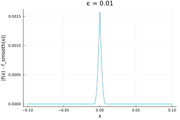
On my machine execution time for invoking f_smooth(x, ϵ) ranges from about 200 nsec for x < ϵ to about 3.5 usec for x > ϵ.

Edit:
Maybe this approach can be cheap enough (on average), since you only need evaluate the smoothed function within the transition region:

f_smoothfaster(x, ϵ) = abs(x) < ϵ ? fsmooth(x, ϵ) : f(x)
3 Likes

While cool, you can also get arbitrarily accurate and analytic without needing to integrate with f(x,ϵ) = log1p(exp(x/ϵ))*ϵ
image

7 Likes

Another alternative; we have {\sqrt{x^2 + b} + x} = {{\sqrt{b}} \cdot {e^{asinh{\frac{x}{\sqrt{b}}}}}}, so there are now three alternatives for squareplus:

squareplus_wikipedia(x, b) = (x + sqrt(x*x + b))/2

squareplus_timholy(x, b) = b/(2 * (sqrt(x*x + b) - x))

function squareplus_exp_asinh(x, b)
  sb = sqrt(b)
  exp(asinh(x/sb))*sb/2
end
3 Likes