Simple curve fitting with CurveFit (or alternative)

I’d like to try different curves against data to see which of them would best fit. So in this example

x0 = collect(1.0:100.0)
y0 = x .^ 4.5
f0 = curve_fit(LinearFit, x0, y0)

I’d like to learn just how bad it is, but is there an easy way to get that out of it?

1 Like

Please check this post.

1 Like

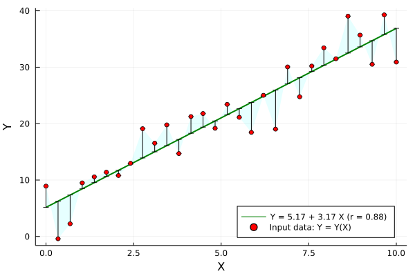
Just in case it might be useful, sharing one linear regression example below, where the correlation coefficient r is displayed and other regression statistics are computed too:

using Plots, Random, Distributions, GLM, DataFrames, Printf

# input data
n = 30
x = LinRange(0,1, n) .* 10
e = rand(Normal(0,mean(x)/4),n)
parms = Dict(:b0 => 6, :b1 => 3.2)
y = parms[:b0] .+ parms[:b1] .* x .+ 3*e
data = DataFrame(X=x, Y=y)

# linear regression
ols = lm(@formula(Y ~ 1 + X), data)
a, b = coef(ols)
r = r2(ols)

# plotting
yhat = parms[:b0] .+ parms[:b1] .* x
err = y - yhat; z0 = 0*err;
str = "Y = " * @sprintf("%.2f",a) * " + " * @sprintf("%.2f",b) * " X (r = " * @sprintf("%.2f",r) * ")" 
plot(x,yhat, label=str, lw=2, c=:green, yerror=(z0,err), ribbon=(z0,err), fc=:cyan, fa=0.1)
scatter!(x, y, mc=:red, xlabel="X", ylabel="Y", label="Input data: Y = Y(X)", legend=:bottomright)

Some stats output after command:

julia> ols = lm(@formula(Y ~ 1 + X), data)

Y ~ 1 + X

Coefficients:
───────────────────────────────────────────────────────────────────────
               Coef.  Std. Error      t  Pr(>|t|)  Lower 95%  Upper 95%
───────────────────────────────────────────────────────────────────────
(Intercept)  5.16706    1.31032    3.94    0.0005    2.48298    7.85113
X            3.172      0.225023  14.10    <1e-13    2.71106    3.63294

linear_regression_with_corr_coeff

2 Likes

Thanks, I’ll look into these examples. The problem itself should be relatively simple, the actual data is a straight line in a log-log plot, it’s just not quite that easy to post its code here. (The wikipedia page for log-log plots is also somewhat opaque.)

Check out this document too on lin-log and log-log regressions.

1 Like

I have a very simple package to make fits really, really simple, in common cases: GitHub - m3g/EasyFit.jl: Easy interface for obtaining fits for 2D data

2 Likes

Just for fun:
To fit a polynom you can use

"""
Fit y = f(x) to nth order polynomial.
Returns list of polynomial coefficients.
"""
function polyfit(x,y,n)
	@assert length(x) > n
	A = [k^n for k in x, n in 0:n]
	A\y
end

To reason about the fit you would need to look for measures often found under goodness of fit, but I am not sure which are implemented by julia packages. If you want to look into one of those methods I think the package HypothesisTests is a good resource.

Also if you try to fit a log transformed exponential function you should use a weighted least square fit to compensate for the transform.

1 Like

Don’t do this — the Vandermonde matrix is generally ill-conditioned.

3 Likes

I got this working with minimal effort (on the package side, I had some other unrelated Julia problems though). When I take log10 of the original x and y values, and do fit = fitlinear(x_log,y_log), I get a nice match.


I can also see that the average square residue is low.

 ------------------- Linear Fit ------------- 

 Equation: y = ax + b 

 With: a = -0.9999071242153111
       b = 5.319512210970783e-5

 Pearson correlation coefficient, R = 0.9999734052571524
 Average square residue = 9.731441862500589e-6

 Predicted Y: ypred = [2.999774567768043, 2.6987725305011243...
 residues = [-0.0008626824944601985, -0.007119649365998182...

 -------------------------------------------- 
1 Like

When I tried to fit against the original (non-log) data, the only one that gave good results was fit = fitspline(x,y).


It’s just that spline doesn’t really tell me anything useful.

 -------- Spline fit --------------------------- 

 x spline: x = [0.001, 0.011...
 y spline: y = [1005.2007999999998, 90.34990000000002...

 ----------------------------------------------- 

A spline will always look well, but you cannot use them to really get any information about your data.

If your x and y values are related by something like y = A/x it is expected that the log/log plot is linear (log(y) = A - log(x)) while the plot of the original data is not.

Yes. X ^ -1 is close. Can I fit that with EasyFit?

No, I didn’t implement that (you can fit anything using directly LsqFit). Although the approach of fitting a straight line in the log/log plot is the best approach. Linear fits are always better.

2 Likes

LsqFit seems to be more general and conveniently provides the confidence intervals for the parameters estimated.
A correlation coefficient might also be obtained from the approximation of the covariance matrix. An attempt below, r formula to be confirmed.

PS: in your case it is possible and better to work with a log-log scale.

using LsqFit, Plots, Printf

# input noisy data
t = 0.01:0.01:1
y = 420*t.^(-0.13 .+ 0.02*rand(length(t)))

# LsqFit
m(t, p) = p[1] * t.^(-p[2])
p0 = [0.5, 0.5]
fit = curve_fit(m, t, y, p0)
# fit parameters and confidence interval
p = fit.param
confidence_interval(fit, 0.1)   # 10% confidence intervals

# correlation coefficient = covariance of 2 variables / product of their standard deviations
cov = estimate_covar(fit)
r = cov[1,2]/sqrt(cov[1,1]*cov[2,2])   # TODO: confirm formula

# plot results
str = @sprintf("%.1f",p[1])*"*t^(-" * @sprintf("%.3f",p[2]) * ")" * @sprintf(";   r ~ %.2f",r)
scatter(t,y, mc=:reds, ms=3, xlabel="t", label="input data")
plot!(t,m(t,fit.param),ly=0.25,lc=:blue, ylabel="y(t)", label="LsqFit: "*str)
julia> p = fit.param
 419.2404632519413
   0.12214587254371537

julia> confidence_interval(fit, 0.1)   # 10% confidence intervals
 (418.14933388256867, 420.331592621314)
 (0.12055572549189375, 0.12373601959553698)

julia> r = cov[1,2]/sqrt(cov[1,1]*cov[2,2])  # TODO: confirm formula
-0.7431633567883187

power_law_LsqFit

1 Like

After thinking about this, I agree. The linear plot is really hard to read if you want any useful info out of it. The only reason against the log-log plot is that I’m not so used to such plots. Well, time to learn.

I’ll take a look at the solutions a bit later.

Also, if this was a part of a machine learning problem, trying gradient descent on the linear data would be a lost cause. I ’knew’ that already, but visualizing it makes is clearer.

If you can linearize the plot, you probably should do the linear fit and afterwards recover the non-linear parameters from that fit.

Now, how you maybe using this for optimizing anything is another story. The function 1/x is also minimum at x -> infty, thus minimizing it or the linearized version will take you to the same place.

How would I get the lin-lin equation from this log-log fit? I spent some reading of the wikipedia page, but not enough to fully get it.

Ok, got it. To change from log-log to lin-lin one can do:
y₂ = MathConstants.e .^ ( a .* log.(x) .+ b .* log.(10))

I did use WolframAlpha, I fed it log10(y) = a * log10(x) + b
It says the answer is approximate form. I then changed it to Julia form.

log₁₀y == a * log₁₀x + b 
10 ^ log₁₀y == 10 ^ ( a * log₁₀x + b )
y == 10 ^ ( a * log₁₀x + b )
y == 10 ^ ( a * log₁₀x ) * 10 ^ b
magic..
y == MathConstants.e .^ ( a .* log.(x) .+ b .* log.(10))

Above is pseudo-code.

Indeed. That can be written in Julia as:

y2 = exp(fit.b) * x.^fit.a

(where fit.b and fit.a are the intercept and slope of the linear fit of the log-log plot - with base e. If you use base 10, use log10, and then y_2 = 10^{fit.b} x^{fit.a}.

1 Like