Hi all, I will be presenting a Julia tutorial on an international PHD school, and OrdinaryDiffEq.jl will be one of the packages I will be highlighting. I want to demonstrate some of the various solvers of the ecosystem via approachable examples. I will showcase two examples: 1) using Tsit5, then going from Tsit5 to Vern9 for better performance when high accuracy is in demand. 2) An example where a stiff solver leads to a better (more stable / more performant) solution. I couldn’t find a simple stiff example in the online docs. Ideally I would like a low dimensional ODE where it makes a big impact to use a stiff solver vs. a non-stiff. Does anyone have an example in mind?
Should contain suitable examples, which are even already preprogrammed ![]()
Specifically, the Robertson or the van der Pol examples may be what you are looking for.
I tend to like user ROBER (Robertson).
https://docs.sciml.ai/SciMLBenchmarksOutput/stable/StiffODE/ROBER/
It is very clearly not possible to solve with explicit methods, just try it. And you can easily see the time scale separation from the coefficients being orders of magnitude apart.
https://docs.sciml.ai/SciMLBenchmarksOutput/stable/StiffODE/VanDerPol/
Van Der Pol is indeed a great example too because it has tunable stiffness. As you change μ you change the time scales and you can see the behavior get more and more smooth. The stuff benchmark we have is from Hairer’s book and uses 1e6, while MATLAB has an example of nonstiff ODEs
which is Van Der Pol at μ=1. This highlights that the difference can be not just structural but also dependent on parameter values.
I would say slow fast systems with relaxation oscillations are likely to show case this.
The Van der Pol example is very appealing to me because the audience I am teaching to will likely be familiar with it, and they are also interested in timescale separation. However, I am having difficulty constructing an example where the stiff solver is “more appropriate”. I’ve cooked up:
function vanderpol_rule(u, μ, t)
    x, y = u
    dx = y
    dy = μ*((1-x^2)*y - x)
    return SVector(dx, dy)
end

fig = Figure()
axs = [Axis(fig[i, :]) for i in 1:2]
algs = (Tsit5(), Rodas5P()) # second is stiff solver

for (i, alg) in enumerate(algs)
    for μ in (1, 1e3, 1e6)
        prob = ODEProblem(vanderpol_rule, SVector(1.0, 1.0), (0.0, 10.0), μ)
        sol = solve(prob; alg, abstol = 1e-12, reltol = 1e-12, saveat = 0.01, maxiters = typemax(Int))
        t = 0:0.01:10
        lines!(axs[i], t, sol[1, :])
    end
end
fig
I was hoping that in this MWE the solutions using Tsit5 would fail or diverge but they don’t, provided that I use large enough maxiters. Is this really all there is to it? that the stiff solvers are just much more efficient in solving these problems and hence take less steps overall?
EdIT: output figure is:
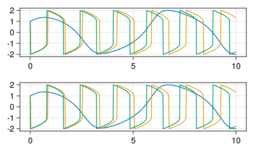
Actually it gets even weirded: I started printing the number of rejected steps, sol.stats.nreject and saw that the stiff solver rejected much more steps:
Alg: Rodas5P, rejected steps: 1551
vs
Alg: Tsit5, rejected steps: 0
for same large μ and same tolerances.
ah okay, but the Rodas solver is much more performant:

thanks a lot @ChrisRackauckas , I’ll use the Van der Pol as an example!!!
Yes, and you can see this for example in the Filament PDE example.
https://docs.sciml.ai/SciMLBenchmarksOutput/html/MOLPDE/Filament.html

An explicit method can take a billion steps to try and solve it, it just takes 50x as long.
Though note that some cases are about stability. ROBER is pretty hard (if possible) to make stable with an explicit method.