I am trying to learn Julia and I read this article about the quick success of Julia. In the last page of the article the author works a small example showing the benefits of multiple dispatch. They define a custom class Spect and define a plot() function for it. Then for an object sqw of type Spect they can call plot(sqw) without having to edit the original plot function. Moreover, this definition also affects similar plotting functions so that you can also call scatter(sqw) without problems. My issue is that author does not show the code, so I do not understand how can you achieve this. I am specially interested in the fact that just defining plot() for this new class is enough to also call other functions like scatter() without defining them for the new class.
Can someone write a small example of this like that of the article so that I can understand how all of this is achieved? Thank you in advance.
It’s a shame the article doesn’t link to the code. Here’s my rough reproduction attempt. My version uses the dct and idct so I’m not getting the nice harmonics, but I think it shows the ideas pretty well.
using RecipesBase, FFTW
struct Spect
    points :: AbstractRange
    weights :: Vector{Float64}
end
function Spect(f::Function, min, max, n)
    points = range(min, max, n)
    Spect(points, dct(f.(points)))
end

@recipe function f(S::Spect)
    S.points, idct(S.weights)
end
These definitions are enough for
using Plots
squarewave(x) = iseven(floor(x)) ? 1.0 : 0.0
sqw = Spect(squarewave, 0, 5, 20);
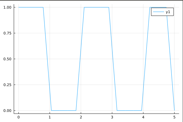
plot(sqw)
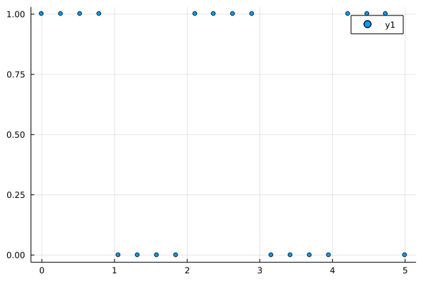
scatter(sqw)
The result of this is
and
This reproduces the figures in the article:
using Plots, RecipesBase

"""Do the Fourier synthesis. a and b are vectors of coefficients for the sine and
cosine components. Return a function of the independent variable."""
function fsc(a, b, x)
     function f(x)
       ss = sum(a .* sin.(x .* (1:length(a))))
       cs = sum(b .* cos.(x .* (1:length(a))))
       ss + cs
     end
     return f(x)
end

"""A datatype that holds two vectors of Fourier components."""
struct Spect
     a::Array{Float64, 1}
     b::Array{Float64, 1}
end

"""The plotting recipe takes a Spect and plots it in physical space."""
@recipe function f(s::Spect)
           x = pi/50 .* (0:100)
           y = map(w -> fsc(s.a, s.b, w), x)
           x, y
        end

#Here is the spectrum of a square wave. It has only odd sine components that
#go as 1/n. Here we include the first 10 harmonics.
a = isodd.(1:10) ./ (1:10)
b = zeros(10)

sqw = Spect(a, b)

#Making the plots. Any function from Plots.jl that understands recipes will
#now be able to plot a Spect.
plot(sqw)
scatter(sqw)

"""Filter a Spect by zeroing anything higher than the nth harmonic."""
function lowpass(s::Spect, n)
     t = deepcopy(s)
     t.a[n+1:end] .= 0
     t.b[n+1:end] .= 0
     return t
end

#Filter the square wave that we created above, keeping only the first three
#harmonics.
filtered_sqw = lowpass(sqw, 3)

#Take a look at the filtered square wave.
plot(filtered_sqw)