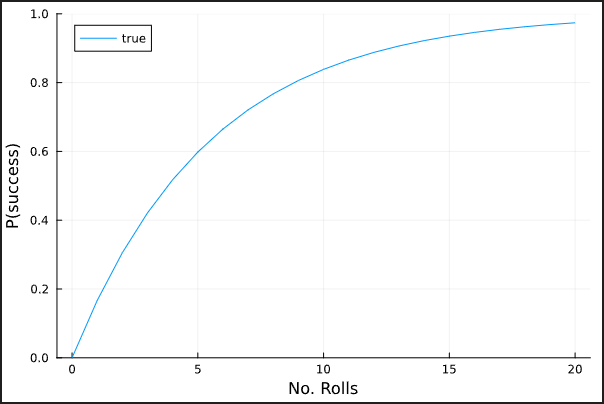
Assume the following: I repeat a game over and over in which I roll a die a number of times. If I roll a 6 on any of the trials, I win. Otherwise, I lose. I want to model how the probability of winning this game changes as the number of trials increases.
In this case, I obviously know the answer when I’m using a standard 6-sided die:
using StatsPlots
# probability of rolling a six on a single throw
p = 1/6
# probability as a function of N (number of rolls)
P(N) = 1 - (1 - p)^N

plot(
	P,
	0:20;
	ylims=(0,1),
	label="true",
	xlabel="No. Rolls",
	ylabel="P(success)"
)
Let’s assume, though, that I do not know the probability of success for a given trial and I do not know how this probability is related to the number of trials. I just have data that show how many trials I ran during each round, and whether or not I won:
using DataFrames
using Distributions

data = DataFrame(num_rolls = rand(5:14, 300))
data.success = [rand(Binomial(row.num_rolls, p)) > 0 for row in eachrow(data)]

300×2 DataFrame
 Row │ num_rolls  success
     │ Int64      Bool
─────┼────────────────────
   1 │        10     true
   2 │        12    false
   3 │        11     true
   4 │        14     true
   5 │        10     true
  ⋮  │     ⋮         ⋮
 297 │         7     true
 298 │         5     true
 299 │         7    false
 300 │         5     true
          291 rows omitted
An important note here is that I’ve deliberately chosen N to be a random number between 5 and 14, since that results in an average success rate of roughly 80%, most of the time.
Since the variable of interest is binary, logistic regression is a common choice. I implement it as follows:
using StatsFuns
using Turing

@model function success_model(success, num_rolls)
	α ~ Normal(-5, 0.1)
	β ~ Normal(0, 1.5)
	for i ∈ eachindex(success)
		p = logistic(α + β * num_rolls[i])
		success[i] ~ Bernoulli(p)
	end
end
I’ve used a really strong prior for my intercept term since I know that the probability of success is zero when the number of rolls is zero. Now I fit my model and compare its average predictions across different values of N to the actual values:
m = success_model(data.success, data.num_rolls)
chain = sample(m, NUTS(), 1_000)
chaindf = DataFrame(chain)
ᾱ = mean(chaindf.α)
β̄ = mean(chaindf.β)
plot(
	P,
	0:20;
	ylims=(0,1),
	label="true",
	xlabel="No. Rolls",
	ylabel="P(success)"
)

plot!(
	x -> logistic(ᾱ + β̄ * x),
	0:20,
	label="model"
)
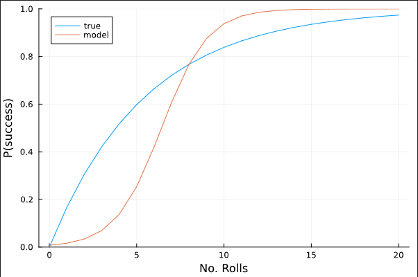
As you can see, this is a pretty terrible model. My next thought was to get rid of the strong prior on the intercept term, so I did that by simply increasing the standard deviation to 2:
@model function success_model(success, num_rolls)
	α ~ Normal(-5, 2)
	β ~ Normal(0, 1.5)
	for i ∈ eachindex(success)
		p = logistic(α + β * num_rolls[i])
		success[i] ~ Bernoulli(p)
	end
end
Now, I have this:
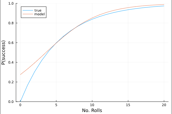
This is a lot better, but still not very satisfying. This model is telling me I have a nonsensical 25% chance (roughly) of success if I don’t roll the die a single time. I’ve played around with different priors for the intercept term and there seems to be this tradeoff between having the model be grounded in reality when N = 0, and having it produce accurate results for higher values of N. I also tried dropping the intercept term completely, and that wasn’t good either. In addition to that, I tried balancing the data by oversampling the values where success == false, again to no avail.
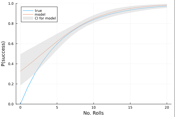
I guess my question is: is there a better link function I can use that will give a more accurate representation of my true underlying model? Or, is it simply a matter of being aware that predictions are less accurate for lower values of N? I can visualize a confidence interval for the average probability of success across different values of N and see that the model has less confidence at lower values of N:
μ = [
	logistic(row.α + row.β * x)
	for row in eachrow(chaindf), x in 0:20
]
μ̄ = [mean(c) for c in eachcol(μ)]
μ₉₀ = hcat([percentile(c, [5,95]) for c in eachcol(μ)]...)'

plot!(
    0:20,
    [μ̄ μ̄],
    fillrange=μ₉₀,
    labels=["CI for model" ""],
    color=:lightgrey,
    alpha=0.5,
    linewidth=0,
)
Or, lastly, is it just a matter of choosing wisely the threshold value that is used when using the model for prediction tasks? I would love to hear thoughts/advice/feedback on how to model this kind of problem. I have a real-world problem that is loosely analogous to this example and it’s pretty scary knowing I can get such dramatically different results, depending on my choice of a prior. I thought I was doing the right thing with the strong prior for the intercept, since I know for sure that there is no chance of success when N = 0, but I see in this example that doing so results in a really terrible fit.
