Quantifying "damping" rate of ODE

Hi,

I’m trying to figure out a way to compare how fast the oscillations in two ODE models decay. For example, the two figures below show the solution of a model that differs only in temperature, and I want to be able to say something like “the model stabilizes faster at higher temperatures” or vis versa. I will be doing this over a range of temperatures for potentially tens of thousands of parameter combinations.


I’ve tried just comparing the coefficient of variation, but that seems to be sensitive to the length of the simulation and certain transient dynamics. I’ve also thought of measuring time until equilibrium (to some level of tolerance), but some combinations of parameters will blow up the model if it runs too long. Perhaps there is a way to fit a negative exponential to the peaks or something? Or maybe there is an easy and established way of doing this in Julia that I just don’t know of. Any help would be greatly appreciated. Thanks!

This sounds like the sort of thing you could do via linearization, if the ODE models are time-invariant.

That is, if you have an ODE like dx/dt = f(x), then in the limit of small \Vert x \Vert (for the asymptotics of a decaying solution), you could approximate this by dx/dt = Jx + f(0), where J is the Jacobian f'(0)… Assuming f(0) = 0 (if the system is decaying to zero), then the decay rate is simply given by the eigenvalue of J with the largest real part (presumably negative for decaying solutions).

It’s the same thing if it’s decaying to some non-zero equilibrium x_0, but then you need to first solve the nonlinear equation f(x_0) = 0 to find the equilibrium x_0 of your model, and then linearize around this — i.e. J is now the Jacobian evaluated at x_0.

This is essentially the same thing as linear stability analysis, which you can find described in many textbooks and sources online.

3 Likes

This sounds like a great idea. I will give it a try as soon as I can. Thanks!

Another approach would be to fit an exponentially damped sinusoid to your data using e.g. Prony’s Method

1 Like

You could also check this other post about computing the Hilbert envelop.

1 Like

This turned out to be a great solution, thank you!

For those interested, I ended up doing this to get the eigenvalue with largest real part.:

     using ForwardDiff, NonlinearSolve
     function stability(inits, parameters) #initial conditions and parameters
        NLprob = NonlinearProblem(Alpha_Temp_B, inits, parameters)  # find roots of model Alpha_Temp_B(u,p)
        NLsol = solve(NLprob, NewtonRaphson())  # find the steady-state
        J = ForwardDiff.jacobian(u -> Alpha_Temp_B(u, parameters), NLsol.u)  # get Jacobian
        max_real = maximum(real.(eigen(J).values)) #get eigenvalue with maximum real part
     end

I had previously found convenient code to do this here: Incorrect bifurcation diagram bifurcationkit.jl - #4 by dawbarton

2 Likes

Thanks for the other suggestions as well. I’ve never heard of Prony’s Method or the Hilbert Envelope, but these are good to know about and could come in handy in the future.

Minor side note: If you only care about the eigenvalues, I would recommend using eigvals(J) rather than eigen(J).values. The reason is that there are more efficient algorithms to compute just the eigenvalues (eigvals) than to compute both eigenvalues and eigenvectors (eigen).

3 Likes

For my own edification, I decided to try to implement what I suggested. I used the matrix pencil algorithm from this paper, which is said to be superior to Prony’s method, after translating the code from Matlab to Julia. I tried fitting a pair (p=2) of complex exponential functions (because the original data is real) to the “tail” of the time series digitized from the first plot in the OP. The minimum time (abscissa) chosen to begin the “tail” was set to 500, 1500, 2000, 2500, and 3000. The resulting quality of fits and computed attenuation constants are shown below.

18°C500

18°C1000

18°C1500

18°C2000

18°C2500

18°C3000

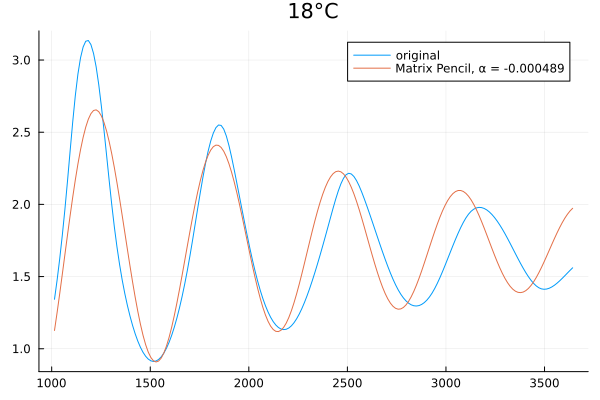
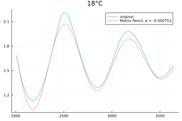
It appears from the last several plots that the attenuation constant is approximately 0.001 neper/sec (assuming the original time unit was seconds). But it’s possible that the system hasn’t yet approached its ultimate decay rate. Since it’s difficult to know a priori how far out in time to solve the system, it’s quite clear to me that the algorithm suggested by @stevengj is definitely the better way to approach this problem. (No surprise there! :wink:)

In case people are interested, here is the listing for the matrix pencil algorithm:

using LinearAlgebra: eigvals, pinv
using ToeplitzMatrices: Hankel

"""
    matrix_pencil(x::AbstractVector, p::Int, Δt::Real) -> (amp, α, f, θ)

Matrix pencil algorithm for fitting a time series with a sum of complex exponentials:

`` x(t) ≈ \\sum_{k=1}^{p} amp[k] * exp((2π*f[k]*im + α[k])*t + im*θ[k]) ``

# Input Arguments
- `x`: Time series sampled at a constant increment.
- `p`: Number of damped exponentials to be identified.  For a real input `x`, `p` should be even.
- `Δt`: The time increment between samples.

# Return Values
- `amp`: Vector of amplitudes of length `p`.
- `α`: Vector of attenuation constants (units are nepers times the inverse of those of `Δt`).
- `f`: Vector of frequencies (units are the inverse of those of `Δt`).
- `θ`: Vector of phase constants (radians).

# Reference
This function is a translation to Julia by Peter S. Simon of the Matlab code 
provided in the Open Access article Fernández Rodríguez, A., de Santiago Rodrigo, 
L., López Guillén, E. et al., "Coding Prony’s method in MATLAB and applying it 
to biomedical signal filtering", BMC Bioinformatics 19, 451 (2018), 
https://doi.org/10.1186/s12859-018-2473-y.
The article is distributed under the terms of the Creative Commons Attribution 4.0 
International License (http://creativecommons.org/licenses/by/4.0/), which permits 
unrestricted use, distribution, and reproduction in any medium, provided you give
appropriate credit to the original author(s) and the source, provide a link to the 
Creative Commons license, and indicate if changes were made. No additional restrictions
are placed on the Julia code by its author.
"""
function matrix_pencil(x::AbstractVector, p::Int, Δt::Real)
    p > 0 || error("p must be a positive integer")
    N = length(x)
    Y = Hankel(x[1:N-p], x[N-p:N])
    Y1 = Y[:, 1:end-1]
    Y2 = @view Y[:, 2:end]

    l = eigvals(pinv(Y1) * Y2)
    
    α = log.(abs.(l)) ./ Δt
    f = angle.(l) ./ (2π * Δt)

    Z = zeros(Complex{real(eltype(x))}, N, p)
    for i in eachindex(l)
        factor = one(eltype(l))
        for k in 1:N
            Z[k, i] = factor
            factor *= l[i]
        end
    end

    for i in eachindex(Z)
        zr, zi = real(Z[i]), imag(Z[i])
        isinf(zr) && (zr = typemax(zr) * sign(zr))
        isinf(zi) && (zi = typemax(zi) * sign(zi))
        Z[i] = complex(zr, zi)
    end

    h = Z \ x
    amp = abs.(h)
    θ = angle.(h)

    return (amp, α, f, θ)
end
5 Likes

That’s a very interesting method! It may come in handy at some point. Thanks for sharing!

1 Like

One quick follow up question, if you don’t mind. Is it possible to obtain information on the amplitude of oscillations from the eigenvalues/vectors of the Jacobian in this case?

This will depend on the initial condition

1 Like

True, but given a set of initial conditions can one determine the amplitude from the eigenvalues? I definitely need to learn the theory better, but I thought perhaps the imaginary parts of the eigenvalues held some information about amplitude, as they do about frequency.

The eigenvalue will determine the frequency and the decay rate, but those are not enough to determine the amplitude. For instance, no matter what eigenvalues you have, if you start in the origin, the amplitude is going to be zero.

I see, very good point. Thanks!