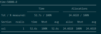
Yes I’m saving 2500 points to check if the orbits is fine. Sometimes I just need the last point than I save the last point.
I tried to use StaticArrays however i’m not sure what i was doing wrong or if it’s even possible use in systems like this.
In that case i’m solving the CR3BP equations with the variational equations and a chaotic indicator
For 5e3 periods of my orbit i’m getting 2.47GB memory usage avg
For 5e4 periods its 24.6GB

Perhabs its already maximum optimized but i’m not sure. i’ll share my code down there.
using Plots, LinearAlgebra, Random, DataFrames, TimerOutputs, StaticArrays, DifferentialEquations

const to = TimerOutput()

@inline @inbounds function vy0(C,p,v)
   """
   Calculate Vy0 from jacobian value
   input : (C,p,v) ...
            C = Jacobi cte
            v = x,y,vx
            p = mass ratio parameters mu
   """
       #cartesian coordinates
       x, y, x̂= v
       #distance vectors
       r1 = ((x+μ)^2 + y^2)^(1/2)
       r2 = ((1-x-μ)^2 + y^2)^(1/2)
       #jacobi integral - constant C.
       ŷ = (x^2 + y^2 - x̂^2 + 2*((1-μ)/r1 + μ/r2) - C)^(1/2)
       return ŷ
end


"""
Initial Conditions
"""
global μ = 0.01 # mass ratio binary main system

# third body
CJ = 0 # Jacobi cte
x0 = 1.893
y0 = 0
vx0 = 0
vyu = -vy0(CJ,μ,[x0,y0,vx0]) #sign negative for retrograde orbits


"""
Create a random set of tangent vector for MEGNO
Get normalized vectors for MEGNO
"""
rng = MersenneTwister(234);
a1 = rand!(rng, zeros(4))
global dd = 0
for i in 1:length(a1)
	if a1[i] <= 0.5
		a1[i] = -a1[i]
	end
end
for i in 1:length(a1)
	global dd += a1[i]^2

end
dd = sqrt(dd)
for i in 1:length(a1)
a1[i]= a1[i]/dd
global dd += a1[i]^2
end


####################
"""
u0 state vector = [x0,y0,vx0,vy0,xrng,yrng,vxrng,vyrng,megno_mean,megno_final]
x0,y0,vx0,vy0 -> Third body

%%%% MEGNO - REFERENCE : https://www.aanda.org/articles/aa/pdf/2001/41/aah2931.pdf
xrng,yrng,vxrng,vyrng = random initial conditions to calculate megno with variational equations
megno_mean = mean value of (dot var_equations / var_equations)
megno_final = numerical integration of the MEGNO mean value
"""
u0 = [x0, y0, vx0, vyu, a1[1], a1[2], a1[3], a1[4], 0.0, 0.0] # vector with initial conditions
println("Initial state vector :",u0)
println("JacobiCte Initial :",CJ)
# Time Span
t_end = 2*pi*5e4
tspan=(0.0,t_end)
numberofpoints = 2500


@inline @inbounds function cr3bp_rhs(du,u,μ,t)
"""
Planar Circular Restricted 3body problem
Equations of motion in co-rotating frame

	in:
		u = position and velocities of the particle
		μ = mass ratio parameter == μ2
		t = time span
	out:
		du = integration of the acel. and vel.

"""

	#cartesian coordinates

	r1 = ((u[1] + μ)^2 + u[2]^2)^(1/2)
    r2 = ((-1 + u[1] + μ)^2 + u[2]^2)^(1/2)

	du[1] = u[3] # F1
    du[2] = u[4] # F2
    du[3] =  2*u[4]  + u[1] - (1 - μ)*(μ + u[1])/(r1^3) - μ*(-1 + μ + u[1])/(r2^3) # F3
    du[4] = -2*u[3]  + u[2] - (1 - μ)*u[2]/(r1^3)       - μ*u[2]/(r2^3) # F4

	# renormalizing tangent vectors everystep for MEGNO - Chaotic Indicator
	normvec = sqrt(u[5]^2 + u[6]^2 + u[7]^2 + u[8]^2)
	xm = u[5]/normvec
	ym = u[6]/normvec
	vym = u[7]/normvec
	vxm = u[8]/normvec

	# mass parameters
	mu1 = 1 - μ
	mu2 = μ
	#derivatives f3
	df3x = 1.0-mu1/r1^3-mu2/r2^3+3.0*mu1*(u[1]+mu2)^2/r1^5+3.0*mu2*(u[1]-mu1)^2/r2^5
	df3y = 3.0*mu1*(u[1]+mu2)*u[2]/r1^5+3.0*mu2*(u[1]-mu1)*u[2]/r2^5
	df3vx = 0
	df3vy = 2

	#derivatives f4
	df4x = 3.0*mu1*(u[1]+mu2)*u[2]/r1^5+3.0*mu2*(u[1]-mu1)*u[2]/r2^5
	df4y =  1.0-mu1/r1^3-mu2/r2^3+3.0*mu1*(u[2])^2/r1^5+3.0*mu2*(u[2])^2/r2^5
	df4vx = -2
	df4vy = 0

	du[5] = vxm
	du[6] = vym
	du[7] = df3x*xm + df3y*ym + df3vx*vxm + df3vy*vym
	du[8] = df4x*xm + df4y*ym + df4vx*vxm + df4vy*vym
	#megno evolve
	f = u[5]*du[5] + u[6]*du[6] + u[7]*du[7] + u[8]*du[8]
	d2 = u[5]^2 + u[6]^2 + u[7]^2 + u[8]^2

	# megno equations
	if t==0 # need check at t=0 to avoid overflows caused by 0 on the denominator
		chaosind1 = (f/d2) * (t + 1e-16)
		du[9] = chaosind1
		du[10] = 2*u[9]/(t + 1e-16)
	else
		chaosind1 = (f/d2) * t
		du[9] = chaosind1
		du[10] = 2*u[9]/t
	end

end

# solver
p = μ
prob = ODEProblem(cr3bp_rhs,u0,tspan,p)
@timeit to "sol" solution2 = solve(prob,Vern9(),reltol = 1e-16,abstol = 1e-16, maxiters = 1e8, saveat = t_end/numberofpoints)

df = DataFrame(solution2)
println("points:",length(df.timestamp))
println("time:",df.timestamp[end]/(2*pi))

"""
Checking if the cte error increases through the time
"""
jacobicte = []
for i in 1:length(df.timestamp)
	x= df.value1[i]
	y= df.value2[i]
	vx= df.value3[i]
	vy= df.value4[i]
	r1 = ((x + μ)^2 + y^2)^(1/2)
	r2 = ((-1 + x + μ)^2 + y^2)^(1/2)
	jacobi = (x^2 + y^2 - vx^2 - vy^2 + 2*((1-μ)/r1 + μ/r2))
	append!(jacobicte,jacobi)
end

p1 = scatter(df.timestamp,jacobicte, label="Jacobi Constant")
p2 = scatter(df.value1,df.value2)
print_timer(to::TimerOutput)
#p4 = plot(df.value9)
np= []
np2 = []

for i in 1:length(df.timestamp)
	b= df.value10[i]/df.timestamp[i]
	append!(np,b)
end


p3 = plot(df.timestamp,np, label=" MEGNO <Y>",  legend=:bottomright)
println("FINAL MEGNO: ", np[end])
plot(p1,p2,p3)

