Hi all,
I want to plot the possible outcomes of tossing a fair coin for n times. If three times tossed then it should be like this graph:
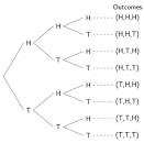
Which package in Julia can make this kind of graph?
Hi all,
I want to plot the possible outcomes of tossing a fair coin for n times. If three times tossed then it should be like this graph:
Which package in Julia can make this kind of graph?
You could use GraphMakie.jl in the Makie or GraphRecipes.jl in the Plots ecosystem.
However I think using Julia plotting libraries makes the most sense when you’re plotting data. Your example looks like you want to explain a concept with a curated graphic, for that I’d recommend to go for a tool like tikz or inkscape rather than a plotting lib.
I want to use Julia so it can calculate the probability and the outcome sets too.
Tikz is possible to graph it, but how about the numerical part? if I want to toss a coin 10 times. Julia should be able to calculate it fast with another package right?
Yes, if you want to visualize a specific sample it makes sense to use a plotting lib. I think you can get fine results using both mentioned packages.
In your original post the graphic includes all possible outcomes for 3 throws, without any “dynamic” data, which is why I suggested a more static approach.
To get the probabilities, you can use the analytical expression:
P_k(n) = \choose{k}{n} \cdot \left(\frac{1}{2}\right)^n
or
probability(k, n) = nchoosek(n, k)*(1//2)^n
I can’t find the perfect sentences so people could understand what I want. If it is finish I will post it here.
Thanks for the reply!
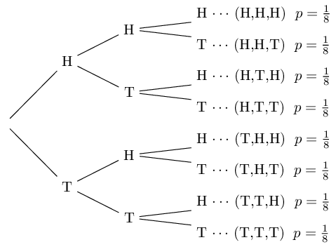
I suppose that you intend to vizualize the binary tree, associated to the experiment consisting in n independent Bernoulli trials. A Bernoulli trial has two mutual exclusive outcomes: success and failure. The probability p of the succes is the same any time when you repeat the trial. In your case p=1/2. In an experiment with n independent trials one is interested in the number if successes (or failures). The random variabile X that records the number k of successes in n trials has the Binomial distribution, and P(X=k)={n \choose k} p^k (1-p)^{n-k}. In your case is given by the formula given by @gustaphe.
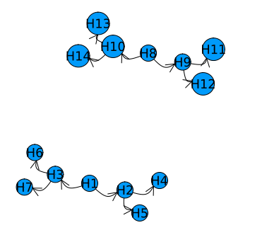
I have tried with an ugly graph like this:
using GraphRecipes, Plots
gr()
default(size=(800, 400))

g = [0  1  1  0  0  0  0  0  0  0  0  0  0  0;
     0  0  0  1  1  0  0  0  0  0  0  0  0  0;
     0  0  0  0  0  1  1  0  0  0  0  0  0  0;
     0  0  0  0  0  0  0  0  0  0  0  0  0  0;
     0  0  0  0  0  0  0  0  0  0  0  0  0  0;
     0  0  0  0  0  0  0  0  0  0  0  0  0  0;
     0  0  0  0  0  0  0  0  0  0  0  0  0  0;
     0  0  0  0  0  0  0  0  1  1  0  0  0  0;
     0  0  0  0  0  0  0  0  0  0  1  1  0  0;
     0  0  0  0  0  0  0  0  0  0  0  0  1  1;
     0  0  0  0  0  0  0  0  0  0  0  0  0  0;
     0  0  0  0  0  0  0  0  0  0  0  0  0  0;
     0  0  0  0  0  0  0  0  0  0  0  0  0  0;
     0  0  0  0  0  0  0  0  0  0  0  0  0  0;]
graphplot(g, fontsize=12, names="H".*string.(1:14), nodeshape=:circle)
The problems:
H,T won’t workI might be able to use Tikz to draw the wanted image, but I think Julia should be able to do it too.
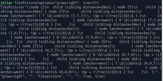
One possibility is to use Julia to generate the TikZ code:
using TikzPictures

function branch(result, n, i=1, prev=[])
    sofar = [prev; result]
    indent = "  "^i
    distance = 5 * 2^(n-i)
    if i == n
        fullbranch = join(sofar, ",")
        prob = "\$p = \\frac{1}{$(2^n)}\$"
        return  """
                $(indent)child [sibling distance=$(distance)ex]
                $(indent)  { node [anchor=west] { $result \$\\cdots\$ ($fullbranch)\\; $prob } }"""
    else
        return  """
                $(indent)child [sibling distance=$(distance)ex] { node {$result}
                $(branch(:T, n, i+1, sofar))
                $(branch(:H, n, i+1, sofar))
                $(indent)}"""
    end
end

function tree(n)
    return """
           \\node {}
           $(branch(:T, n))
           $(branch(:H, n));"""
end

TikzPicture(options="grow=right", tree(3))
To define a binary tree of depth h=3, the adjacency matrix must have the size (15,15). Your matrix is (14, 14). This function creates the ajacency matrix of a perfect binary tree of depth h:
function get_adjacency(h::Int)
    nn = 2^(h+1)-1 #number of nodes
    A = zeros(Int64, nn, nn);
    j=2
    for i = 1:2^h-1
        A[i, j] = 1
        A[i, j+1] =1
        j=j+2
    end
    return A
end
To assign a position to each tree node, install NetworkLayout.jl. Then with:
using Graphs, NetworkLayout
A = get_adjacency(3)
G = DiGraph(A);
node_pos = buchheim(G.fadjlist)
you get a binary tree placed vertically. By default, the root is at the point (0,0). To get an horizontally displayed tree, rotate the points in the vector node_pos around the root with an angle of π/2. The rotation matrix is [0 -1; 1;0].
Having the new node position you can now plot the corresponding binary tree.
I didn’t know the logic behind matrix of size (15,15) for h=3, thanks @empet . I just go with my own thinking for matrix 14x14.
Julia is amazing
Wow @sijo this is what I am looking for. Thanks a bunch!
I get this when run the code at REPL:
why it won’t show the image?
The REPL cannot show images… You should see the image if you run the code in a Jupyter notebook. Or if you save the result in a variable tp, you can call save(PDF("filename"), tp) to output a PDF file (see the TikzPictures.jl documentation for more details),
(To put the image here on Discourse I used the Linux convert tool to convert the PDF to PNG.)
The adjacency matrix of a graph has the size (nn, nn), where nn is the number of nodes. Now count the nodes in the above plotted binary tree and you get 15.
I think I have to put L """ in the right place, the pdf generated but it is empty:
using TikzPictures

function branch(result, n, i=1, prev=[])
    sofar = [prev; result]
    indent = "  "^i
    distance = 5 * 2^(n-i)
    if i == n
        fullbranch = join(sofar, ",")
        prob = "\$p = \\frac{1}{$(2^n)}\$"
        return  """
                $(indent)child [sibling distance=$(distance)ex]
                $(indent)  { node [anchor=west] { $result \$\\cdots\$ ($fullbranch)\\; $prob } }"""
    else
        return  """
                $(indent)child [sibling distance=$(distance)ex] { node {$result}
                $(branch(:T, n, i+1, sofar))
                $(branch(:H, n, i+1, sofar))
                $(indent)}"""
    end
end

function tree(n)
    return """
           \\node {}
           $(branch(:T, n))
           $(branch(:H, n));"""
end


tp = TikzPicture(L""" options="grow=right", tree(3)""")

save(PDF("test"), tp)
No you shouldn’t add any L: all the dollars and backslashes in my code are already escaped. So replace
tp = TikzPicture(L""" options="grow=right", tree(3)""")
with
tp = TikzPicture(options="grow=right", tree(3))
and it should work.
Following the steps I outlined above, I defined the binary tree associated
to a Bernoulli experiment consisting in 4 trials. 1 encodes the trial success, while 0, the failure.
The outcomes of this experiment are 4-length bitstrings returned by this function:
function bit_strings(h::Int)
   #returns the vector of h-length bitstrings
   vbstr = String[]
   for i = 0:2^h-1
       s = bitstring(Int8(i)) #Int8 is sufficient for h=4, 5, 6, 7
       push!(vbstr, s[length(s)-h+1:end])
   end
   return vbstr
end
I tried with Jupyter Notebook too why this code can’t work ? Neither REPL nor notebook works.
My Julia: version 1.7.3
status:
Status `~/LasthrimProjection/Test/Project.toml`
  [bd48cda9] GraphRecipes v0.5.12
  [86223c79] Graphs v1.8.0
  [95701278] ImplicitEquations v1.0.9
  [b964fa9f] LaTeXStrings v1.3.0
  [f0f68f2c] PlotlyJS v0.18.10
  [91a5bcdd] Plots v1.38.0
  [438e738f] PyCall v1.94.1
  [d330b81b] PyPlot v2.11.0
  [1fd47b50] QuadGK v2.6.0
  [24249f21] SymPy v1.1.7
  [37f6aa50] TikzPictures v3.4.2

This one has a great blend of colors black and yellow!
Thanks a lot @empet .
I agree with binary results. 1 0 is the machine code anyway

