Piecewise-constant fitting

rafael.guerra · February 5, 2023, 1:45pm

Is there an example or a Julia package for piecewise-constant fitting of 1D series?

See a Matlab example of expected results here.

Thanks.

stevengj · February 5, 2023, 2:03pm

See Interpolations.Constant

rafael.guerra · February 5, 2023, 2:20pm

@stevengj, thanks. Does the fact that it uses the nearest-neighbor imply that it might be a bit off from the expected mean?

stevengj · February 5, 2023, 2:42pm

What is the “expected mean”?

If you have data from x\in [a,b], and an interpolated function f(x), do you want the continuous mean \frac{1}{b-a} \int_a^b f(x) dx to be something in particular? What? (If you say “I want it to equal the mean of the discrete data points”, stop and think about what this means for the endpoint weighting.) Nearest-neighbor piecewise-constant interpolation corresponds exactly to a trapezoidal rule integration.

stevengj · February 5, 2023, 2:45pm

Oh, I see — what you want is not piecewise-constant interpolation, but rather piecewise constant least-square fitting. This seems similar to this question, so probably you can use related techniques: Piecewise linear regression with automatic knot selection

rafael.guerra · February 5, 2023, 2:47pm

Thanks, I have edited the title to not upset the mathematicians

In any case, I will test the suggested constant interpolation.

dlakelan · February 5, 2023, 5:51pm

If you’re doing least squares why would you want piecewise constant? Why not just use a Chebyshev Polynomials or a Radial Basis Function or similar? Unless you think the underlying function is itself constant and measured with noise I guess.

rafael.guerra · February 5, 2023, 5:53pm

One application: modelling layered media with layers of constant properties and variable thickness. Where the input data is experimental and continuous, not necessarily noisy. Actually, estimating some optimum K break points is the most important part.

RoyiAvital · February 5, 2023, 6:24pm

If you’re OK with simple translation from MATLAB, take the code I wrote in matlab - Deconvolution of a 1D Time Domain Wave Signal Convolved with Series of Rect Signals - Signal Processing Stack Exchange. Just use H = I or optimize the code specifically to this case.

This matches the optimization problem in your link.
Yet this is not a Piece Wise Fitting, It is Least Squares with TV regularization which means the prior is a function with sparse derivative. It means it promotes piece wise constant signals.

By the way, for piece wise linear, just adapt the D matrix to calculate the 2nd derivative.

rafael.guerra · February 5, 2023, 11:55pm

I am copying further below some input data to play with and one example of what might be one piecewise-constant result for K=21 break points:

Input 1D series (400 equidistant points)

Dan · February 6, 2023, 12:08am

Isn’t it possible to write the JuMP/Optimization equivalent of the problem from the MATLAB link?

cvx_begin
    variable x(n)
    minimize( sum_square(y-x) )
    subject to
       norm(D*x,1) <= K;
cvx_end

from: https://inst.eecs.berkeley.edu/~ee127/sp21/livebook/exa_pw_fitting.html
as noted in OP.

odow · February 6, 2023, 1:01am

There are a few options with JuMP.

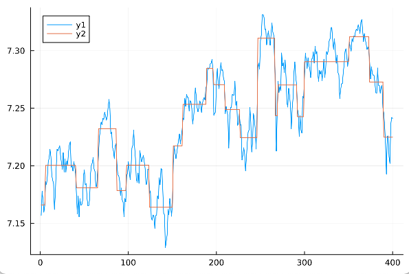
using JuMP, Gurobi, Plots
K = 21
δ = maximum(y) - minimum(y)
model = Model(Gurobi.Optimizer)
set_time_limit_sec(model, 30)
@variables(model, begin
    x[1:N]
    z[1:N], Bin
end)
@constraints(model, begin
    sum(z) <= K - 1
    [i=2:N], x[i] - x[i-1] <= z[i] * δ
    [i=2:N], x[i] - x[i-1] >= -z[i] * δ
end)
@objective(model, Min, sum((y .- x).^2));
optimize!(model)
plot(y)
plot!(value.(x))

@Dan’s CVX equivalent is:

using JuMP, Gurobi, Plots
N = length(y)
D = zeros(N-1, N);
for i in 1:(N-1)
  D[i, i] = -1
  D[i, i+1] = 1
end
K = 0.25
model = Model(Gurobi.Optimizer)
@variable(model, x[1:N]);
@objective(model, Min, sum((y .- x).^2));
@constraint(model, [K; D * x] in MOI.NormOneCone(N))
optimize!(model)
plot(y)
plot!(value.(x))

You have to tune K a bit. It doesn’t represent the number of break points.

rafael.guerra · February 6, 2023, 1:09am

Thanks for the good stuff, the top solution looks brilliant.

Is it possible to constrain it to have a minimum distance between breakpoints, to avoid very short steps? Perhaps as an alternative criteria to fixed K.

Regarding:

This guy needs special installation. Why do we need it? Are there any alternatives?

odow · February 6, 2023, 1:25am

Is it possible to constrain it to have a minimum distance between breakpoints, to avoid very short steps?

Yes. Constrain z so that it can change value only once in a given window:

window = 10
@constraint(model, [i=window:N], sum(z[i-j+1] for j in 1:window) <= 1)

This guy needs special installation. Why do we need it? Are there any alternatives?

If you’re an academic you can get a free license. We need a mixed-integer quadratic solver. There aren’t many great free alternatives.

If you use the L1 norm for the loss function instead of the L2, then you can use HiGHS:

using JuMP, HiGHS, Plots
K = 21
δ = maximum(y) - minimum(y)
model = Model(HiGHS.Optimizer)
set_time_limit_sec(model, 30)
@variables(model, begin
    x[1:N]
    z[1:N], Bin
    t
end)
window = 10
@constraints(model, begin
    sum(z) <= K - 1
    [i=window:N], sum(z[i-j+1] for j in 1:window) <= 1
    [i=2:N], x[i] - x[i-1] <= z[i] * δ
    [i=2:N], x[i] - x[i-1] >= -z[i] * δ
    [t; y .- x] in MOI.NormOneCone(1 + N)
end)
@objective(model, Min, t);
optimize!(model)
plot(y)
plot!(value.(x))

rafael.guerra · February 6, 2023, 1:34am

Thank you, this is brilliant.

I like the L1 norm results too.

dlakelan · February 6, 2023, 2:17am

You could do a nice Bayesian model in Turing. A prior on the distance between nodes, a Normally distributed error, and a prior on the jump sizes, then cumsum the x values and the Y values… You’d get a comprehensive sample of plausible fits.

PeterSimon · February 6, 2023, 5:33am

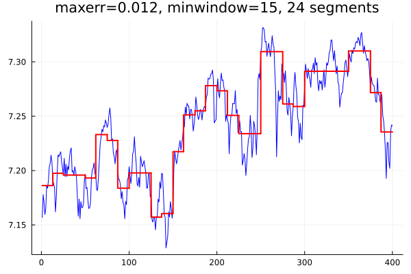
I know you have a solution already, but I wanted to see if I could work this problem without using sophisticated optimizers. Here is my effort:

using Statistics

struct Segment{T}
    x1::T
    x2::T
    y::T
end

function piecewiseconst(x::AbstractVector, y::AbstractVector, maxerr::Real, minwindow::Int=10)
    length(x) == length(y) || error("x and y have unequal lengths")
    ymid, ymax = quantile(y, (0.5, 0.8)) 
    value = ymid
    err = ymax - ymid
    segment = Segment(x[begin], x[end], value)
    if err ≤ maxerr || length(x) < max(minwindow, 3)
        return [segment]
    else
        bind = firstindex(x)
        eind = lastindex(x)
        mind = (bind + eind) ÷ 2
        l = piecewiseconst(view(x, bind:mind), view(y, bind:mind), maxerr, minwindow)
        r = piecewiseconst(view(x, mind:eind), view(y, mind:eind), maxerr, minwindow)
        return vcat(l, r)
    end
end

The function returns a Vector{Segment} comprising the piecewise constant approximation to the input data. Here is how to apply it to your data and plot the result:


using Plots, DelimitedFiles

ypts = readdlm("sampledat.txt")[:]
xpts = [float(i) for i in 1:length(ypts)]

function plotit()
    p = plot(xpts, ypts, color=:blue, legend=:none)
    yold = ypts[begin]
    for (i, s) in enumerate(segs)
        x1, x2, value = s.x1, s.x2, s.y
        if i == 1
            x = [x1, x2]
            y = [value, value]
        else
            x = [x1, x1, x2]
            y = [yold, value, value]
        end
        plot!(x, y, color=:red, lw=2)
        yold = value
    end
    plot!(p, title = "maxerr=$maxerr, minwindow=$minwindow, $(length(segs)) segments")
    display(p)
end

maxerr = 0.012
minwindow = 15
segs = piecewiseconst(xpts, ypts, maxerr, minwindow)
plotit()

The resulting plot looks like this:

plot

jd-foster · February 8, 2023, 1:04pm

For interest (I like the elegance of the integer optimisation approach) your method reminded me of a principle put forward by de Boor that:
pwc_deBoor

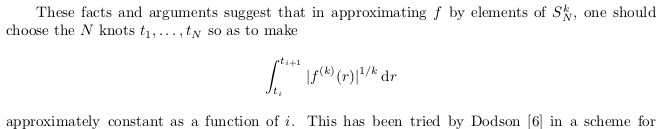
The below implements this idea fairly simply (for k = 1 in the equation above):

using DelimitedFiles, Statistics

# Set number of segments
K = 21

# Get data:
y_data = readdlm("sampledat.txt")[:]
N = length(y_data)
x_data = 1:N

# Define breakpoints / knots (include the endpoints)
t = zeros(Int,K+2) # To be determined
t[begin] = 1
t[end] = N

# Define function values over segments
f = zeros(K+2)     ## To be calculated
f[begin] = y_data[begin]
f[end] = y_data[end]

y_diff = [abs(y_data[n+1] - y_data[n-1]) for n in 2:(N-1)]

# Sum of absolute values of data:
S = sum(y_diff)

# Constant contribution on each segment:
T = S/(K+1)
C = cumsum(y_diff)
t[(begin+1):(end-1)] = [Int(argmin(abs.(C .- k*T))) for k in 1:K]

# The best fit value over a single segment is the mean:
for i in 1:K+1
    f[i] = mean(y_data[t[i]:t[i+1]])
end

Plotting code:

using Plots

function plot_pwc_data(indices,values)

    x = [indices[begin]]
    y = [values[begin], values[begin]]
    
    for i in 2:(length(indices)-1)
        push!(x, indices[i], indices[i])
        v = values[i]
        push!(y, v, v)
    end
    push!(x, indices[end])
    
    return x, y
end

p = plot(x_data, y_data, color=:blue, legend=:none)
plot(p)

tt, ff = plot_pwc_data(t,f)

plot!(tt, ff, color=:red, lw=2)

rafael.guerra · February 8, 2023, 8:34pm

@PeterSimon & @jd-foster, thanks for the nice out-of-the box ideas, which provide food for thought.

@jd-foster, btw, plot_pwc_data() could be conveniently replaced by:
plot!(t, f, lt=:step, c=:red, lw=2)

stephenll · February 8, 2023, 9:30pm

What about the Pelt algorithm for id’ing change points? “Optimal detection of changepoints with a linear computational cost.”