Hello!
Lately I am always getting an error when simulating a ModelingToolkit.jl model with uncertain parameters from Measurements.jl. I have the feeling that this worked before and the error especially came up after upgrading Julia from 1.8 to 1.9 but I am not exactly sure.
My code is the following:
using ModelingToolkit
using DifferentialEquations
using Measurements
@variables t
D = Differential(t)
@mtkmodel batchferm1 begin
@parameters begin
	μ_max = 0.6 ± 0.1
	k_s = 0.05
	Yₓ = 0.45 ± 0.1
end
@variables begin
	X(t)
	S(t)
	μ(t)
end
@equations begin
	D(X) ~ μ * X
	D(S) ~ - μ / Yₓ * X
	μ ~ μ_max * S / (k_s + S)
end

@mtkbuild batch1 = batchferm1()
prob1 = ODEProblem(batch1,
		[batch1.X => 0.3,
		batch1.S => 10.0],
		(0,7.5));
sol = solve(prob1, Tsit5(), reltol=1e-6, abstol=1e-6)
I am getting the following error:
MethodError: no method matching Float64(::Measurements.Measurement{Float64})
Closest candidates are:
(::Type{T})(::Real, !Matched::RoundingMode) where T<:AbstractFloat
@ Base rounding.jl:207
(::Type{T})(::T) where T<:Number
@ Core boot.jl:792
(::Type{T})(!Matched::AbstractChar) where T<:Union{AbstractChar, Number}
@ Base char.jl:50
Note, that you get a very poor approximation to the uncertainty in the solution using linear uncertainty propagation, the code below allows you to switch to nonlinear uncertainty propagation by redefining the ± and the difference is rather big
using ModelingToolkit
using Plots
using OrdinaryDiffEq

import Measurements, MonteCarloMeasurements

± = Measurements.:(±) # Pick one or the other
± = MonteCarloMeasurements.:(∓)

@parameters t
D = Differential(t)
@mtkmodel batchferm1 begin
    @parameters begin
        μ_max = 0.6 ± 0.1
        k_s = 0.05
        Yₓ = 0.45 ± 0.1
    end
    @variables begin
        X(t)
        S(t)
        μ(t)
    end
    @equations begin
        D(X) ~ μ * X
        D(S) ~ - μ / Yₓ * X
        μ ~ μ_max * S / (k_s + S)
    end
end

@mtkbuild batch1 = batchferm1()
tspan = (0,7.5)
prob1 = ODEProblem(batch1,
		[batch1.X => 0.3 ± 0,
		batch1.S => 10.0],
		tspan);
sol = solve(prob1, Tsit5(), reltol=1e-6, abstol=1e-6)

t = range(tspan..., length=100)
plot(t, sol(t, idxs=1).u, layout=2, sp=1)
plot!(t, sol(t, idxs=2).u, sp=2)
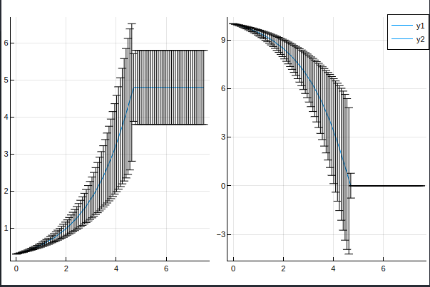
Linear:
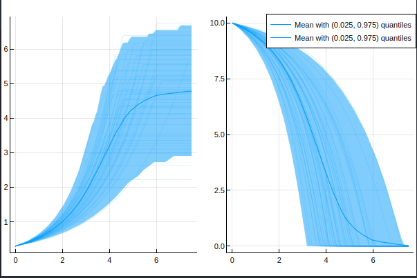
Nonlinear:
In particular, the linear version
gives zero uncertainty for the second variable after t \approx 5
severely underestimates the uncertainty for the first variable after the same time point
Says that it’s possible for the second variable to be negative
So if this problem is representative of what you would like to do, it would probably be wise to interpret the result with caution.
Wow thanks a lot! Yes I already encountered that and thought nonlinear propagation might be better especially because of the highly nonlinear behaviour at about 5 h (batch end) … but I had no idead that this is so easy to achieve
All of the entries will be promoted to the closest common supertype, and standard floats thus promotes to uncertain numbers if at least one number is uncertain.
The initial condition is used to determine the element type of the integrator state.