Say we have discrete CDF values (percentiles from the field for one metric) such as
percentile 1 => 1.4
…
percentile 10 => 10.3
…
percentile 50 => 50.3
…
percentile 80 => 70.3
…
percentile 100 => 90.3
I am construction a CDF using linear interpolation such as
percentile_values = [
[0.0, 0.01, 0.1,
1.0, 2.0, 3.0, 4.0, 5.0, 6.0, 7.0, 8.0, 9.0,
10.0, 20.0, 30.0, 40.0, 50.0, 60.0, 70.0, 80.0,
90.0, 91.0, 92.0, 93.0, 94.0, 95.0, 96.0, 97.0, 98.0, 99.0,
99.9, 99.99, 100.0]

using Interpolations
Xs = [...] # same length as percentile_values

nodes = (percentile_values,)
itp = interpolate(nodes, Xs, Gridded(Linear()))
Questions:
- Can i generate PDF from this interpolated function using differentiation ? If so can you help me with sample code ?
- I have attached standalone sample code that describes my current process ( code uses quantiles [0,1] instead of percentiles [0,100] just to adhere to CDF rules), can you suggest more robust process to convert information from CDF to PDF ?
- Can you provide suggestions an comments on the current method used by me using
Spline1D?
Please refer sample code
using Dierckx
using Interpolations
using ImageFiltering
import Plots
import StatsPlots
using Plots.PlotMeasures
Plots.gr()
Plots.theme(:ggplot2)
# sample input
q_values = [ 0.0, 0.0001, 0.001,
0.01, 0.02, 0.03, 0.04, 0.05, 0.06, 0.07, 0.08, 0.09,
0.1, 0.2, 0.3, 0.4, 0.5, 0.6, 0.7, 0.8, 0.9,
0.91, 0.92, 0.93, 0.94, 0.95, 0.96, 0.97, 0.98, 0.99,
0.999, 0.9999, 1.0 ]
feature_values = [ 9.0, 12.0, 14.0,
23.0, 28.0, 31.0, 33.0, 36.0, 38.0, 39.0, 41.0, 43.0,
45.0, 58.0, 70.0, 80.0, 87.0, 91.0, 94.0, 95.0, 97.0,
97.0, 97.0, 97.0, 97.0, 97.0, 97.0, 98.0, 98.0, 98.0,
99.0, 99.0, 100.0 ]
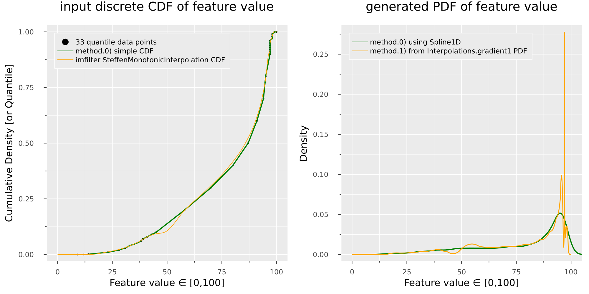
# TODO task: Generate PDF from discrete quantiles (also called discrete CDF)
p1 = Plots.scatter(feature_values, q_values, markersize=1.75, color="black", label="33 quantile data points")
Plots.plot!(p1, feature_values, q_values, label="method.0) simple CDF",
title = "input discrete CDF of feature value", color=:green, linewidth=2,
ylabel="Cumulative Density [or Quantile]",
xlim=(-5,105), xlabel="Feature value ∈ [0,100]",
border=nothing
)
# using Spline1D
# interpolate function mapping quantiles -> feature values
spl = Spline1D(q_values, feature_values, k=1, bc="extrapolate")
sample_cdf_q_values1 = [rand() for p in 1:25000]
pdf_of_feature_values1 = [evaluate(spl, p) for p in sample_cdf_q_values1]
p2 = Plots.density(pdf_of_feature_values1,
title = "generated PDF of feature value", color=:green, linewidth=2, label="method.0) using Spline1D",
ylabel="Density",
xlim=(-5,105), xlabel="Feature value ∈ [0,100]",
border=nothing
)
# using methods from Interpolations
# https://discourse.julialang.org/t/interpolations-jl-discrete-cdf-to-pdf/60124/8?u=bicepjai
# smoothing to get a more reasonable-looking PDF
smoothed_feature_values = imfilter(feature_values, ImageFiltering.Kernel.gaussian((1,)));
sample_feature_values = 0.01:0.01:100.0 # just a range for plotting
# you can change SteffenMonotonicInterpolation to some other monotonic algorithm from Interpolations.jl
itp_cdf = extrapolate(interpolate(smoothed_feature_values, q_values, SteffenMonotonicInterpolation()), Flat());
Plots.plot!(p1, sample_feature_values, itp_cdf.(sample_feature_values),
color=:orange, linewidth=1, label="imfilter SteffenMonotonicInterpolation CDF")
itp_pdf(x) = Interpolations.gradient1(itp_cdf, x); # this is the PDF generate
Plots.plot!(p2, sample_feature_values, itp_pdf.(sample_feature_values),
color=:orange, linewidth=1.5, label="method.1) from Interpolations.gradient1 PDF")
# using new methods update the plots with different colors
# so that its easier for comparision
l = @Plots.layout([ a{0.5w} b{0.5w} ])
Plots.plot(p1, p2, layout=l,
legend=:topleft,
top_margin=5mm, bottom_margin=5mm, left_margin=5mm,
dpi=200, size=(1000,500), fmt = :png
)
References:
update: sample code and plots