'Initial condition incompatible' error w/ DifferentialEquations.jl

Hello all,
I am trying to solve a stiff ODE using DifferentialEquations.jl and am running into an error that says Initial condition incompatible with functional form.
Here is the equation I am trying to solve:

Here is the code:

using DifferentialEquations, Plots

# Constants
const M = 135e3 # MPa # 135 GPa
const R_star_pipe = (10^(-0.95))  # MPa-5 s-1
const Q = 453000  # J/mol
const R = 8.314   # J/mol k
const T = 1573 # in K
const EXP = 2.718^(-Q/(R*T))
const R_star_gb = 10^(3.53)  # MPa-4 s-1
const A = 10^6.94 # MPa-2 s-1
const d = 400.0^1e-6 # grain size in micrometer 
const beta = 2
const mu = 65e3 #MPa #65 GPa
const b = 5 * (10^-10) # in meters


function backstr!(dS, S, p, t)
    sigma_tmax, sigma_d, sigma_ref, sigma = p
    St = S
    epsilon_dot = A*EXP*(St^2)*sinh((sigma-St-sigma_d)/sigma_ref)
    dS[1] = (M( (St+sigma_d)*epsilon_dot/St - St*abs(epsilon_dot)/sigma_tmax - R_star_pipe*EXP*(St^5) - R_star_gb*(St^3)*sigma_d ))
    nothing
end

params = [1.8e3, beta*mu*b/d, 3.1e3, 100 ]

tspan = (0,10)
St = 1.00
ode_prob = ODEProblem(olivinebackstr!,St,tspan,params)

ode_sol = solve(ode_prob)

Any help will be greatly appreciated.

Your initial condition needs to be a vector.

St = [1.00]

And you were missing a multiplication in the expression for dS[1].

using DifferentialEquations, Plots

# Constants
const M = 135e3 # MPa # 135 GPa
const R_star_pipe = (10^(-0.95))  # MPa-5 s-1
const Q = 453000  # J/mol
const R = 8.314   # J/mol k
const T = 1573 # in K
const EXP = 2.718^(-Q / (R * T))
const R_star_gb = 10^(3.53)  # MPa-4 s-1
const A = 10^6.94 # MPa-2 s-1
const d = 400.0^1e-6 # grain size in micrometer
const beta = 2
const mu = 65e3 #MPa #65 GPa
const b = 5 * (10^-10) # in meters


function olivinebackstr!(dS, S, p, t)
    sigma_tmax, sigma_d, sigma_ref, sigma = p
    St = S[1]
    epsilon_dot = A * EXP * (St^2) * sinh((sigma - St - sigma_d) / sigma_ref)
    dS[1] = (
        M * (
            (St + sigma_d) * epsilon_dot / St - St * abs(epsilon_dot) / sigma_tmax -
            R_star_pipe * EXP * (St^5) - R_star_gb * (St^3) * sigma_d
        )
    )
    nothing
end

params = [1.8e3, beta * mu * b / d, 3.1e3, 100]

tspan = (0, 10)
St = [1.00]
ode_prob = ODEProblem(olivinebackstr!, St, tspan, params)

ode_sol = solve(ode_prob)

@contradict : you have fixed more things… like the name of the function (backstr! → olivinebackstr!).

But there are more problems, I think. Like:

# const EXP = 2.718^(-Q / (R * T))
# should be
const EXP = exp(-Q/(R*T))

And what about:

# const d = 400.0^1e-6
# should probably be
const d = 400e-6

Possibly more.

[400.0^1e-6 is approximately 1. I assume it should be 400 micrometers, which is 400e-6 meters, not micrometers. With this fix, you should use a tspan of (0,1e-6) instead of (0,10)]

Good catch! I didn’t check the numbers at all just that it solved.

Thanks a lot @contradict @BLI.

Ah, you also lack the EXP term in the last term of the differential equation, I think [at least compared to your screenshot of the Backstress equation]:

# ... R_star_pipe * EXP * (St^5) - R_star_gb * (St^3) * sigma_d
# should be
 R_star_pipe * EXP * (St^5) - R_star_gb * EXP * (St^3) * sigma_d

This missing EXP term has a dramatic effect on the solution! Instead of using a time span of (0,1e-6), you need a time span of (0,5e4) or so.

I have no idea what your model is about, but – since you are new in the community, and I like to play around with models, in particular with ModelingToolkit. So I have:

  • implemented your model in ModelingToolkit – just to inspire you to learn that package,
  • used Unicode characters in the equation to make it more similar to the screenshot.

Here is the model implementation + solution using ModelingToolkit:

using ModelingToolkit, DifferentialEquations, Plots
using ModelingToolkit: t_nounits as t, D_nounits as D
#
params = @parameters begin
    R = 8.31,           [description = "Gas constant, in J/(K.mol)"]
    T = 1573,           [description = "temperature, K"]
    Q = 453_000,        [description = "heat of..., J/mol"]
    M = 135e3,          [description = "..., in MPa"]
    R°_p = 10^(-0.95),   [description = "..., 1/(MPa^5.s)"]
    R°_gb = 10^3.53,    [description = "..., 1/(MPa^4.s)"]
    A° = 10^6.94,       [description = "..., 1/(MPa^2.s)"]
    d = 400e-6,         [description = "grain size, m"]
    β = 2,              [description = "..., ..."]
    μ = 65e3,           [description = "..., MPa"]
    b = 5e-10,          [description = "..., m"]
    Exp = exp(-Q/(R*T))
    #
    σ_T_max = 1.8e3
    σ_d = β*μ*b/d
    σ_ref = 3.1e3        # σ∗_p*R*T/Q
    σ = 100
end
#
vars = @variables begin
    σ_T(t) = 1.0
    ϵ°(t) # = A°*Exp*1^2*sinh((σ - σ_T - σ_d)/σ_ref)
end
#
eqs = [ϵ° ~ A°*Exp*σ_T^2*sinh((σ - σ_T - σ_d)/σ_ref),
        D(σ_T) ~ M*( ϵ°*(σ_T + σ_d)/σ_T - abs(ϵ°)*σ_T/σ_T_max - R°_p*Exp*σ_T^5 - R°_gb*Exp*σ_T^3*σ_d )]

@named sys_eq = ODESystem(eqs,t,vars,params)
sys = structural_simplify(sys_eq)

This produces a “typeset” version of the equation:

Finally, a numeric problem can be created based on the symbolic model sys, and solved:

tspan = (0,5e4)
prob = ODEProblem(sys,[],tspan)

sol = solve(prob)

plot(sol, lw=2.5, lc=:blue,legend=:topleft, xlabel="time")
plot!(twinx(), sol, idxs=(ϵ°), lw=2.5, lc=:red, legend=:bottomright,
    xlabel="", title="Backstress")

leading to:

Regarding Unicode characters, e.g., σ is created by LaTeX-style command \sigma + TAB, etc. Symbol ϵ° is created by \epsilon + TAB, followed by \degree + TAB. Although your screenshot seems to use asterisk instead of the “degree” symbol, you can not use \ast in the variable name, because this will be interpreted as multiplication, or something.

1 Like

Thanks @BLI. I had no idea about ModelingToolkit package, will surely look into it.

Note: the above line is a relatively new syntax in ModelingToolkit, and defines symbol t to be time, and symbol D to be time derivative.

ModelingToolkit is a “language” for writing models in a more “symbolic” form, where the order of equations does not matter – the compiler from the symbolic form to the numeric problem is advanced, and simplifies and sorts the equations in the correct order – and converts it to something similar to your olivinebackstr! function. The result is very efficient code without too much thinking. If you are a super coder, you may be able to do it more efficiently, but for most people – the developers of ModelingToolkit are more likely to produce efficient code for you.

Also, ModelingToolkit is very good if you want to re-use code and connect models.

So unless you are a super programmer, I really recommend you to learn and use ModelingToolkit [or: MTK].

Whether one uses Unicode symbols in variable names, is another question. Some people don’t like that; it may complicate things if you don’t have a word processor that supports Unicode. Personally, I am attracted to the idea of Unicode symbols as long as it makes the model description clearer.

Observe that mathematical equality is written as ~ in MTK, the tilde symbol on the keyboard.

I also really recommend to use and fill in the description strings – this is a good way to document your code.

2 Likes

Hi again,

How do I evaluate a symbolics variable at a particular instance for example ϵ° at t=4e4?

I wouldn’t use the phrase “evaluate a symbolics variable”. At this stage, the solutions are available and they are numeric. But anyway, maybe your phrase is ok.

It is important to understand the structure of the solution which I have called sol. The solution contains two fields t and u – field t holds the time instances where the solution has been found, while field u holds the computed values of the unknowns in these time instances.

In the case of Backstress:

> sol.t'     # I use transpose `'` symbol to save vertical space
1×32 adjoint(::Vector{Float64}) with eltype Float64:
 0.0  0.762987  8.39286  84.6916  …  44162.9  45314.9  47666.0  50000.0

> sol.u'
1×32 adjoint(::Vector{Vector{Float64}}) with eltype LinearAlgebra.Adjoint{Float64, Vector{Float64}}:
 [1.0;;]  [1.00003;;]  [1.00033;;]  [1.00329;;]  …  [70.7544;;]  [70.751;;]

Observe that we have found the solution in 32 time instances. Also, observe that sol.u is a vector of vectors. Each element in the vector holds the solution of all unknowns in the corresponding time instance. So as an example, vector element sol.u[3] holds the solution of unknowns corresponding to time sol.t[3]. Two specific points:

  1. Why is there only one unknown with solution in sol.u?
  2. The shape of sol.u is not in a form that can be plotted.

  1. sol.u and unknowns.
    Field u of the solution only holds the solution to variables formally defined as unknowns. To find out which these are, and their order of storage in sol.u, you need to query:
> unknowns(sys)
1-element Vector{SymbolicUtils.BasicSymbolic{Real}}:
 σ_T(t)

What about other “unknowns”? These have been stripped off the model and made into observed variables; the observed variables are found by:

> observed(sys) |> println
Equation
[ϵ°(t) ~ A°*Exp*
sinh((-σ_T(t) + σ - σ_d) / σ_ref)*(σ_T(t)^2)]

I’ll get back to how to compute this observed variable – which is what you ask about, I guess.


  1. The shape of sol.u and how to make it plottable…
    Perhaps the most efficient way to make sol.u plottable is:
> reduce(vcat,sol.u)'    # Again: transpose to save space
1×32 adjoint(::Vector{Float64}) with eltype Float64:
 1.0  1.00003  1.00033  1.00329  …  70.7375  70.7376  70.7544  70.751

Now you have the solution in a vector of elements, and not in a vector of vectors. The same should work if sol.u has multiple unknowns.

Plotting the result can be done by:

plot(sol.t, reduce(vcat,sol.u))

which produces:


Notice how jagged the solution is compared to doing:

plot(sol)

which produces

The reason for the jaggedness in the first method, plot(sol.t, reduce(vcat,sol.u)) , is that this draws straight lines between the datapoints of sol.t[j] and sol.u[j].


One of the fancy things with Julia solvers is that sol not only holds the solution in datapoints, i.e., sol.t, etc. The solution also includes interpolation functions. Interpolation in a certain time point t0 is given by syntax sol(t0), e.g.:

> sol(4e4)
1-element Vector{Float64}:
 70.74021605315112

This is the solution σ_T(t=4e4).

Final question: how can you specify which variable you want to know the value of? And how can you find the value of observed variables? Simple:

> sol(4e4, idxs=σ_T)
70.74021605315112

> sol(4e4, idxs=ϵ°)
3.6413814395589957e-7

> sol(4e4, idxs=[σ_T, ϵ°])
2-element Vector{Float64}:
 70.74021605315112
  3.6413814395589957e-7

What about plotting observed variables (and unknowns) with interpolation?

plot(sol, idxs=σ_T)

produces.

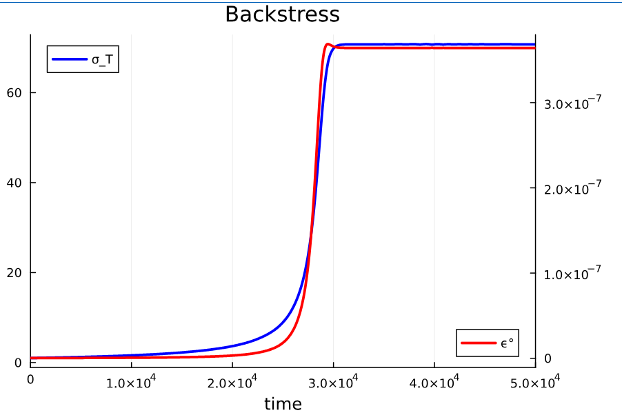
It is also possible to scale time variable and results:

plot(sol, idxs=(t/60,[ϵ°*1e8,σ_T]), label=["epsilon*1e8" "sigma"], xlabel="time [min]", ylabel="")

produces:

If you want a parametric plot of the two dependent variables with time as parameter:

plot(sol, idxs=(σ_T, ϵ°*1e8))

produces:

3 Likes

Thanks for explaining this @BLI it clarifies my question fully.

BTW. The above term is internal stress equation of an Earth mineral Olivine. It depicts in internal behaviour of the mineral under external forces. Further I am working to see if a NeuralODE can learn its behaviour with just a few initial time steps and extrapolate to later ones.

Also, I am quite surprised to see the speed up MTK provides over the vanilla DifferentialEquations package.

Thanks again

Does the response make sense? Is it this slow?

Not fully sure what you mean. But if I understand it correctly, yes the response is making sense and the 1st code w/o MTK is slower.

What I mean is: does the shape of these curves make sense?

  • Doet it take ca. 400 minunetes before sigma_T sharply rises to the sigma_T_max?

Apologies for the late reply. I am still running test on this but for what I can tell the results are looking fine.

Thanks

1 Like