My earlier script was having data race problem. It used to get terminated. Now it is ok. Updated code without lock is ![]()
updated code
using HDF5, GLMakie, Interpolations, Statistics, Profile, Base.Threads, BenchmarkTools
@profile begin
function readhdf(h5file::String)
h5 = h5open(h5file, "r")
B = h5["B"]
@views Br, Bθ, Bϕ = B[:,:,:,:,1], B[:,:,:,:,2], B[:,:,:,:,3]
Bp = @. hypot(Br, Bθ) / Bϕ
x_all, y_all, z_all = h5["x1v"], h5["x2v"], h5["x3v"]
xe_all, ye_all, ze_all = h5["x1f"], h5["x2f"], h5["x3f"]
MeshBlockSize = read((HDF5.attributes(h5))["MeshBlockSize"])
blocks::Int32 = read(HDF5.attributes(h5),"NumMeshBlocks")
return Bp, x_all, y_all, z_all, xe_all, ye_all, ze_all, MeshBlockSize, blocks
end
Bp, x_all, y_all, z_all, xe_all, ye_all, ze_all, MeshBlockSize, blocks = readhdf("sane00.prim.01800.athdf")
function bound(xe_all, ye_all, ze_all, MeshBlockSize, blocks)
XX,YY,ZZ = ntuple(_ -> zeros(Float32, blocks* prod(MeshBlockSize.+1)), 3)
icx=1
for b in 1:blocks
@views r, θ, ϕ = xe_all[:, b], ye_all[:, b], ze_all[:, b]
for rr in r, th in θ, ph in ϕ,
XX[icx] = rr * sin(th) * cos(ph)
YY[icx] = rr * sin(th) * sin(ph)
ZZ[icx] = rr * cos(th)
icx += 1
end
end
xmin,xmax = extrema(XX); ymin,ymax = extrema(YY); zmin,zmax = extrema(ZZ)
println(" x ∈ [$xmin, $xmax], y ∈ [$ymin, $ymax], z ∈ [$zmin, $zmax]")
return xmin, xmax, ymin, ymax, zmin, zmax
end
xmin, xmax, ymin, ymax, zmin, zmax = bound(xe_all, ye_all, ze_all, MeshBlockSize, blocks)
function clp(X,Y,Z,C,xmin,ymin,zmin,sx,sy,sz,nx,ny,nz,field)
xi = trunc(Int, (X-xmin) * sx) + 1
yi = trunc(Int, (Y-ymin) * sy) + 1
zi = trunc(Int, (Z-zmin) * sz) + 1
ix = clamp(xi, 1, nx)
iy = clamp(yi, 1, ny)
iz = clamp(zi, 1, nz)
field[ix, iy, iz] = C
end
function cart(iex,ii,jj,kk,r_eval,θ_eval,ϕ_eval,ext_itp,X,Y,Z,C)
rr, th, ph = r_eval[ii], θ_eval[jj], ϕ_eval[kk]
X[iex] = rr * sin(th) * cos(ph)
Y[iex] = rr * sin(th) * sin(ph)
Z[iex] = rr * cos(th)
C[iex] = ext_itp(rr, th, ph)
end
function loaddata(Bp, x_all, y_all, z_all, xe_all, ye_all, ze_all, MeshBlockSize, blocks)
nx,ny,nz = 10(MeshBlockSize.+1)
field = fill(NaN32, nx,ny,nz)
println("🧩 Allocated $(nx)×$(ny)×$(nz) grid.")
sx = (nx-1)/(xmax-xmin); sy = (ny-1)/(ymax-ymin); sz = (nz-1)/(zmax-zmin)
X, Y, Z, C = ntuple(_ -> zeros(Float32, 1000 * prod(MeshBlockSize.+1)), 4)
@threads for b in 1:blocks
println("Block: $b")
@views r, θ, ϕ = x_all[:, b], y_all[:, b], z_all[:, b]
@views re, θe, ϕe = xe_all[:, b], ye_all[:, b], ze_all[:, b]
@views Bp_block = Bp[:, :, :, b]
ext_itp = extrapolate(interpolate((r, θ, ϕ), Bp_block, Gridded(Linear())), Interpolations.Line())
r_eval = LinRange(re[1], re[end], 10(MeshBlockSize[1]+1))
θ_eval = LinRange(θe[1], θe[end], 10(MeshBlockSize[2]+1))
ϕ_eval = LinRange(ϕe[1], ϕe[end], 10(MeshBlockSize[3]+1))
nr, nθ, nϕ = length(r_eval), length(θ_eval), length(ϕ_eval)
iex::Int32 = 1
@inbounds for ii in 1:nr, jj in 1:nθ, kk in 1:nϕ
cart(iex,ii,jj,kk,r_eval,θ_eval,ϕ_eval,ext_itp,X,Y,Z,C)
clp(X[iex],Y[iex],Z[iex],C[iex],xmin,ymin,zmin,sx,sy,sz,nx,ny,nz,field)
iex += 1
end
end
return X,Y,Z,field
end
X,Y,Z,field = loaddata(Bp, x_all, y_all, z_all, xe_all, ye_all, ze_all, MeshBlockSize, blocks)
function tdplot(xmin, xmax, ymin, ymax, zmin, zmax, field)
finite_vals = filter(!isnan, vec(field))
q_low, q_high = quantile(finite_vals, (0.05, 0.95))
fig = Figure()
ax = LScene(fig[1,1], show_axis=false)
#ax = Axis3(fig[1,1], title="Faster", aspect=:data)
volume!(ax, xmin..xmax, ymin..ymax, zmin..xmax, field, transparency=true; colorrange=(q_low, q_high))
display(fig)
end
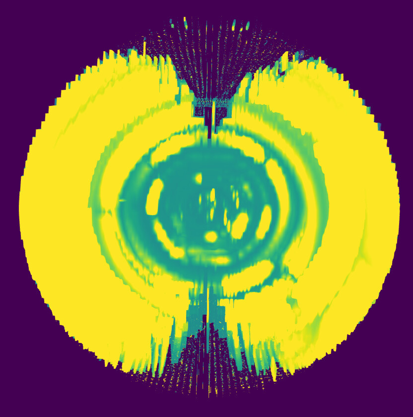
tdplot(xmin, xmax, ymin, ymax, zmin, zmax, field)
end
Profile.print(format=:flat)